Metrical Dimensional Relations of the Aether:

In order to establish the dimensional relations regarding the calculations of the Inductance of the magnetic field, and the Capacitance of the dielectric field, metrical dimensional relations must be applied to the Aether. It is however we really know very little of anything quantitive about this Aether. Names like J.J. Thomson, N. Tesla, G. Le-Bon, W. Crookes, and Mendelev, all have an important role in the Electrical Engineer’s understanding of the aether concept. The physical representation of the Aether as an ultra-fine gas has been qualitivly established, this gas relating to the “Pre Hydrogen Series” of the un-abridged Periodic Table of the Elements. In an analogous compliment is the Trans-Uranium Series of the currently known Periodic Table of the Elements.

This gaseous Aether is the seat of electrical phenomena thru the process of its polarization. This polarization gives rise to induction, which then gives rise to stored energy. Tesla gives a good presentation of his Aether ideas in his “Experiments with Alternate Currents of High Potential and High Frequency.” Given in previous chapters has been the Planck, Q, as the primary dimensional relation defining the “Polarized Aether”, this as an “Atom of Electricity”. It is however, from the views of J.J. Thomson, the Coulomb, psi, the total dielectric induction is the primary dimension defining the “Polarized Aether”. Thomson developed the “Aether Atom” ideas of M. Faraday into his “Electronic Corpuscle”, this the indivisible unit. One corpuscle terminate one one Faradic tube of force, and this quantified as one Coulomb. This corpuscle is NOT and electron, it is a constituent of what today is known as an electron. (Thomson relates 1000 corpuscles per electron) In this view, that taken by W. Crookes, J.J. Thomson, and N. Tesla, the cathode ray is not electrons, but in actuality corpuscles of the Aether. The lawyer like skill of today’s theoretical physicist (Pharisee) has erased this understanding from human memory, it is henceforth sealed by the Mystic Idol of Albert Einstein. If Einstein says no, then it is impossible. What a nice little package.

However, as Electrical Engineers we can give a “Flying Foxtrot” about Einstein, or about bar room fights over the constitution of the Aether. The City of Los Angeles wants its electricity and our job is to get it there intact. How to accomplish this begins with the understanding of Inductance and Capacitance. These represent the energy storage co-efficients of the electric field of induction, this induction in turn a property of the Aether. Magnetic Inductance is thus a dimensional relation for the magnetic properties of the Aether, and Dielectric Capacitance is thus a dimensional relation for the dielectric properties of the Aether. Inductance and Capacitance are thus the application of metrical dimensional relations to certain characteristics of the Aether.

For the magnetic induction the Aetheric relation is known as the magnetic “Permeability”, for the dielectric induction the Aetheric relation is known as the dielectric “Permittivity”. These two terms were so named by Oliver Heaviside. Here the Permeability is denoted as Mu, the Permittivity as Epsilon. These two relations represent the “Magnetic Inductivity” and the “Dielectric Inductivity”, respectively. This pair of dimensional relations, Mu and Epsilon, in conjunction with the metrical dimensional relations defined by the metallic-dielectric geometry bounding the electrified Aether, constitute the dimensional relations of Inductance and Capacitance. It is therefore the Inductance and the Capacitance, L and C are in, and of, themselves metrical dimensional relations. They consist of not substancive dimensions, they are not substantial, they are metrical.

The substancive dimensional relation of Dielectric Induction, psi, in Coulomb, is combined with the metrical relation of Capacitance, C, in Farad, giving rise to the compound dimensional relation of electro-static potential, e, in Volt.

(1) Coulomb, Psi, substantial

Farad, C, metrical

Volt, e, compound, substantial and metrical.

The Farad “operates upon the Coulomb, giving rise to the Volt.

Likewise, the substancive dimensional relation of Magnetic Induction, Phi, in Weber is combined with the metrical dimensional relation of Inductance, L, in Henry, giving rise to the compound dimensional relation of magneto-motive force, I, in Ampere

(2) Weber, Phi, substantial

Henry, L, metrical

Ampere, I, compound, substantial and metrical

The Henry “operates” upon the Weber, giving rise to the Ampere.

The permittivity, as a factor of Capacitance, and the Permeability as a factor of Inductance represent aspects of the medium bounded by the metallic-dielectric geometry. Mu represents the magnetic aspect, Epsilon the dielectric aspect of this medium, be it Aether or 10-C oil. Here it should be noted that the electrical activity is contained solely within the Dielectric Medium, not within the metallic portion of the geometry which bounds it. Again, the basic theory of J.C. Maxwell.

The concept of gradients is here again evoked. These gradients,

(3) Volt per Centimeter, d

(4) Ampere per Centimeter, m

can be represented each in a pair of forms, these giving four gradients total. One form represents the gradient co-linear with the tubes of force themselves, these considered as circuits. The gradients here are in “series”. This condition exists within the “lumped” capacitors and inductors. These gradients constitute “Forces” within the Lines of Induction and can be considered longitudinal in nature.

The alternate form of gradient exists broadside to the tubes of force. Here the inductive forces appear as “fronts” and the gradients can be seen as in “parallel”. This condition exists along the span of the long distance A.C. transmission line. This is,

(5) Volt per Span, d’

(6) Ampere per Span, m’

Here the gradients exist perpendicular or transverse to the Lines of Induction.

Hence, as given, the dielectric gradients, d, and d’, as well as the magnetic gradients, m, and m’, can in general exist each as space quadrature pairs, and as such can represent versor magnitudes in space. See Space Versor part in “Theory of Wireless Power”, by E.P. Dollard. Here again basic electrical relations exist in the archetypal four polar form. The dielectric and the magnetic relations each can be expressed as a pair of versor sub-relations, or four relations total. It may be inferred that both the Inductance and the Capacitance each can be expressed in a pair of distinct forms. This is for (3) and (4) THE “Mutual” Capacitance in per Farad, and the “Mutual” Inductance in per Henry, respectively. For (5) and (6) it is the “Self” Capacitance, in Farad, and the “Self” Inductance, in Henry, respectively. Hereby the four co-efficients of induction,

(I) The Electromagnetic co-efficients;

(a) Self Inductance in Henry, L

(b) Self Capacitance in Farad, C

(II) The Magneto-Dielectric co-efficients;

(a) Mutual Inductance, in Per Henry, M

(b) Mutual Capacitance, in Per Farad, K

The co-efficient, M, may be called the “Enductance” and the co-efficient, K, may be called the “Elastance”. This four polar condition will be considered later on. In what follows will be in terms of the transverse electro-magnetic form, self Inductance and self Capacitance.

The Law of Magnetic Proportion is expressed by the dimensional relation,

(7) Weber, or Ampere – Henry

And for the Law of Dielectric Proportion,

(8) Coulomb, or Volt – Farad

The gradients of the Inductance and the Capacitance, are given as, for the magnetic,

(9) Henry per Centimeter, or Mu,

And for the dielectric,

(10) Farad per Centimeter, or Epsilon.

Hereby taking the Inductance gradient, Mu, and the Capacitance gradient, Epsilon, and substituting these into the Law of Magnetic Proportion and the Law of Dielectric Proportion, respectively, the product of the resulting magnetic and dielectric relations gives

(11) Weber – Coulomb per Centimeter Square

Equals

Volt – Ampere – Mu – Epsilon

Substituting the following relations

(12) Mu – Epsilon, or Gamma Square, (Metric)

(13) Weber – Coulomb, or Planck, (Substancive)

And substituting (12) and (13) into (11) gives

(14) Planck per Centimeter Square, or
Volt – Ampere – Gamma Square

Since it is that

(15) Volt – Ampere equals Planck per Second Square

Substituting (15) into (14) and canceling the Plancks, produces the dimensional relation

(16) Per Centimeter Square

Equals

Per Second Square – Gamma Square

Rearranging this relation, the product (11) gives the definitive metrical dimensional relation

(17) Gamma Square

Equals

Second Square per Centimeter Square

Or thus

(17a) Gamma Square, or one over Velocity Square

And it has been determined that this velocity is the velocity of light. This is to say, the product of the Magnetic Permeability, Mu, and the Dielectric Permittivity, Epsilon, is one over the velocity of light square. This relation is the very foundation of the theory of Electro-Magnetic Wave Propagation thru the Aether, this in a transverse induction form. It is a T.E.M. bounded wave. Hence the product Mu – Epsilon is a fundamental metrical relation of the “Luminiferous Aether”, the carrier of light.

It must be remembered that here it is both Mu and Epsilon represent transverse relations only, and thus useful only in a Transverse Electro-Magnetic metallic-dielectric geometrical form.

Explosion at the Shipyard, N.F.G. :

Lieutenant Junior Grade, U.S.N. Albert Einstein is seated before five senior officers at a Judge Advocate General Board of Inquiry. It has been convened at Pearl Harbor Naval Shipyard. Lt. J.G. Einstein is the defendant and the Board is about to issue it’s verdict. The charges are very serious.

It seems that Mr. Einstein utilized a college physics textbook, in lieu of Bureau of Ships directives, in performing operations on a shore power connection. Mr. Einstein employed “his understanding”, as derived from Physics, “Maxwell’s Equations”, in determining the connections for a shore power transformer bank (480V at 1500 KVA). Seaman Lopez was directed by Lt. J.G. Einstein to make the “backward” connections, but Lopez knew the outcome would spell disaster. He learned in his Naval Electricians Mate training that the connection would cross phase, however Mr. Einstein berated Lopez, as Einstein’s Princeton University education overshadowed “Electricity Schools”. Lopez was reminded that to refuse orders would result in a Captains Mast and possible Court Martial under the U.C.M.J. A terrified Lopez closed the switch and was killed in the blast. Four more were injured and the Shipyard was without power for several hours.

Lieutenant Junior Grade Albert Einstein was pronounced –guilty- by the Board. He received a life sentence at Leavenworth Federal Prison. The next day the Chief of Naval Operations issues the following directive to all Fleet Commanders. It reads in part; At 0000 hours U.T.C. Dec 21, 2012 the following order is in effect: The use of Physics Texts in any and all Naval Operations is henceforth PROHIBITED. The next day a Presidential Order is signed abolishing the practice of teaching Electrical Principles by Physicists. (But the Mayan Calendar says we will not make it that far)

We have reached the Final Proclamation. It can no longer be avoided. It is that the “Laws of Physics” find no application in the understanding of Electricity for the Electrical Scientist. The Physicist is best regarded as a subversive from an enemy country, and his efforts best suited for the development of “Weapons of Mass Destruction.”

The entire system of “Units and Dimensions” for electrical work as they exist today are an incongruous quagmire force fit to Einstein’s E equals mc square. Electricity is a “mass free” phenomena. This is given by Dr. Wilhelm Reich in his “Cosmic Superimposition”. Mass has no place in Electrical Units and a directive is issued to remove it from said units and dimensions. The question of mass is touched upon by Oliver Heaviside in his “Electro-Magnetic Theory” Vol I, pages 337 to 339.

Art. 189, Internal Obstruction and Superficial Conduction
On page 339, “In the limit, with no resistance (perfect conduction) it never gets in at all. Where then is the current?” There is none.

It is further found that the existing system of units are infected with useless constants such as 4*pi and one over c square, as well as a multitude of arbitrary powers of ten. The systems of units as they exist today are pure N.F.G. This is given by Heaviside, same Volume I, pages 116 to 123.

Art. 90, “The eruption of the 4*pi”

Art. 91, “The origin and the spread of the Eruption.”

Art. 92, “The cure of the Disease by Proper Measure of the Strength of the Sources.”

Art. 93, “The Obnoxious Effect of the Eruption.”

Art. 94, “A Plea For the Removal of The Eruption by the Radical Cure.”

Here now the Primary Directive is issued: Rationalize the system of units and dimensions. Remove all “pathogenic” dimensional relations, MASS IN PARTICULAR. This will follow shortly. (Also, on this matter see “Impulses, Waves, Discharges”, Steinmetz, pages 14 & 15.)

Lamare has pushed forward these writings in order to accommodate the “Moon-bounce Initiative”. Hence certain introductory material for the “Youngsters” must be passed over for now. This “act of genius” on the part of Lamare must in itself be pushed forward; An International Ham Contest to disprove Einstein, (but do not ask the A.R.R.L.). Wow Mr. Wizard, that sounds like loads of fun. Lets get started today.

It should be noted however that Lamare is taking a most difficult path. His route lacks any definite engineering formulation but let me draw his attention to C.P. Steinmetz and the treatment of a related situation. It is found in “Theory and Calculation of Transient Electric Phenomena”, “Transients in Space” and section on “Velocity of Propagation of the Electric Field, Capacity of a Sphere”. When the one over c square and the 4*pi*10^-9 are eliminated, the velocity of propagation of the dielectric field is an independent variable. These relations were given by myself at the International Tesla Society in my lecture “Hysteresis of the Aether”. The P.E.E.E., QRM and Dis-infos were conspicuously absent from this presentation! I wonder why?

It is however, that the Telluric Transmission Networks of N. Tesla are completely engineer-able. This is also true for the U.S.N. Alexanderson systems of transmission. The Rogers U.S.N. system also should be noted. The Tesla “thru the Earth” radio has been rendered mere technical details by the writings of L.V. Bewely, Blume, Steinmetz, and Dollard. In particular note Bewely, “Traveling Waves on Transmission Systems,” chapter on single winding waves, and Dollard, “Condensed Introduction to the Tesla Transformer”, and “Theory of Wireless Power” section on coil Coil Calculations. The Tesla Magnifying Transmitter is now an engineer-able reality, this for any competent radio engineer. The 160 meter Ham Band, (1.8 – 2.0 Megacycle per sec.) is the perfect spot for our “International Contest.” My longitudinal videos show the construction of a “160 meter” flat spiral transformer. These medium wave frequencies along with large paths of transmission on a quadrant of the Earth make velocity determination possible. Note that Tesla’s drawing indicates that velocity depends on the cosecant of the latitudinal angle, it is infinity at the poles and luminal at the equator, if anyone ever bothered to look at the fine print. The pi over two is the effective velocity between the limits of c and infinity. There is no longer any excuse for not implementing Tesla Transmission on the Ham Bands, none!

Now the Coyote has to puke. Up comes the goo & mucus of undigestable matter, what a mess. Forget the Bearden fecal matter, Forget the Corum carrion. IT IS ABSOLUTELY USELESS. This material is Pathogenic, also from another standpoint. There are Journalistic Interest, such as the B.B.C. & etc. that sometimes turn a favorable ear to Tesla concepts. For these interested to get mired in a concatenated sequence of falsehoods & misconceptions is the “Kiss of Death” to any public awareness. It also illegitimizes “The Work” in the eyes of Scientists & Engineers. Puke it up once and for all!

The Bearden zealot stands at the bottom of the utility pole, exclaiming to the lineman on top, replacing a missing cross-arm brace, “You lose half your power in that 33KV line (50% efficient) because you don’t pump the Scalar Waves.” The irritated Lineman drops the brace and now must climb down to retrieve it. Angered, the Lineman slams his fist into the mouth of the yac-yac, knocking him to the ground and shouts, “This Line is 98% efficient you moron.” What more can I say, Heaviside E.M. Theory, Vol III, page 1, art. 450.

Adagio. Andante, Allegro Moderato.

“There is a time for all things: for shouting, for gentle speaking, for silence; for washing of pots and the writing of books. Let the pots go black, and set to work. It is hard to make a beginning, but it must be done.” Oliver Heaviside

Prelude, Quadra-Polar Electricity:

It has been repeatedly observed in the previous writings that any given dimensional relation, say Volt, Ampere, and etc always exist in a dual relation. This is known since it is e, in volts and E, in volts. The geometric archetype of the electric phenomena is four polar. This polar quadrantal form is well expressed in Native American art forms. These serve as their “Versor Diagrams” for the four polar seasons and lunar positions. These are important for those that “live outside”. See “When Stars Look Down” for a good popular, not technical, description of this topic. The quadra-polar concept in the mind of Nikola Tesla resulted in the polyphase motors and generators of todays AC technology.

It is likewise, Inductance and Capacitance are a pair of co-efficients representing a pair of fields, and in turn each representative co-efficient in itself exists as a pair, hence giving the four co-efficients total.

Steinmetz first noticed this quadrature pair of inductances in his study of the AC power transformer. This inductance now exists as a pair of inductances: the Leakage Inductance, L, and the Mutual Inductance, M. The lines of induction for L are at right angles (Space Quadrature) to the lines of induction for M. So it is L and M do not “see each other”. Alexanderson utilized this is his magnetic amplifier. Here the saturation flux must be in space quadrature with the power flux. It is then that the two are separated but in the same core. In a metallic-dielectric form it is given as a torroidal magnetic circuit, wound with a pair of metallic circuits, one in winding around the core cross sectional area, the other winding at right angles to the torroidal windings, this being circumferal around the core. (See Alexanderson Patents). Here derived is a “Quadrapolar Inductance Coil”. This quadrapolar inductance, LM, serves as a first step towards understanding tesla type transformers. Needless to say P.E.E.E. Pupin rudely declared Steinmetz as un-Maxwell. So Here we go again.

With regard to parameter variation only the first step has been taken. For example:

Henry per 1, or Henry

Henry per 1 second

That is to say

Henry per second, or Ohm

But what about Henry per second square, or what?

Hueristic (see Guillimen) dimensional relations will be utilized as before.

To quote Maxwell “Electricity and Magnetism” volume 1, page 2;

“A knowledge of the dimensions of the units furnishes a test which ought to be applied to the equations resulting from any lengthened investigation. The dimensions of every term of such an equation, with respect to the three fundamental units must be the same. If not, the equation is absurd, and contains some error, as its interpretation would be different according to the arbitrary system of units which we adopt.”

Here utilized are the “Three Fundamental Units”:

1. Planck

2. Second

3. Centimeter

See “Theorie de Chaleur” by Fourier

Parametric oscillator – Wikipedia, the free encyclopedia

Application of power multiplication to electric power distribution

We have landed, and it is now possible to understand electricity with complete freedom from the shackles of Physics. We are now entering a New World and it is yet to be discovered what wonders may lay ahead.

We have broken the “Einstein Barrier”. He has been left behind on the Prison Planet, but Oliver has been taken with us. We are not done with him yet. No one will live long enough to exhaust the works of Heaviside, and in all probability, Human Society will not either.

The electrical “System of Units and Dimensions” that have been established and taught in the “Schools” of today is encapsulated in a thick coating of E equals mc square, intermingled with the likes of four pi and one over c square, and peppered with a multitude of arbitrary powers of ten. This system is really a complete, absolute, mess.

In order that we may continue to utilize the established size of the Ohm, Volt, Henry, and etc, and remain in accord with the new system of dimensions that has been presented in my series of writings, a mathematical “adapter” must be derived. This adapter will also make lucid the sheer extent of the mess. (See table at end)

Previously established in my writings has been a concrete dimensional system for the description of the “Electrical Phenomena”. These relations will serve as the screws, nuts, and bolts with which to construct a revised concept of electricity, this in accord with the efforts of J.J. Thomson, Oliver Heaviside, Nikola Tesla, and Carl Steinmetz. We no longer need to be involved in the convolutions of the Pendant, the Mystic, and the Dis-informer. They are back on the prison planet with Albert Einstein.

Three dimensions form the primary basis for subsequent relations:

(1) Q, Total Electrification, Planck,

This is our substantial dimension, the spaghetti, or the milk; and,

(2) t, Time, Second,

(3) l, Space, Centimeter.

These serve as our metrical dimensions, the forgotten past, or the throw-away package.

Subsequently established has been a series of dimensions and dimensional relationships, save yet Inductance, Capacitance, and the Electric Force. Two primary substantial dimensions were established by divorce from Q.

(1) Ψ, Total Dielectric Induction, Coulomb,

(2) Φ, Total Magnetic Induction, Weber.

Derived then are four secondary, or compound, dimensional relations:

(1) I, Displacement Current, Ampere,

(2) E, Electro-Motive Force, Volt,

The laws of induction; and,

(3) e, Electro-static Potential, Volt,

(4) i, Magneto-Motive Force, Ampere,

The laws of proportion.

Hereby it is we have two Volts and two Amperes:

Volt; Weber per second, E,

Volt; Coulomb per Farad, e,

And

Ampere; Coulomb per second, I,

Ampere; Weber per Henry, i.

These four dimensional relations serve the principle needs of Electrical Theory.

A pair of auxiliary dimensional relations are also important. These are given as,

(1) Energy; Joules, or Planck per Second

(2) Activity, or Power; Watt, or Planck per Second Square.

Here we have arrived at eight principle dimensional relations for the understanding of Electrical Theory and Practice. All other dimensional relations are developed from consideration of the Metallic-Dielectric Geometry and the Aether with which it is engaged.

In our effort to cleanse the system of units and dimensions, a foremost extraneous element is the “Bogo”, and its arbitrary powers of ten. The Bogo, bs, is entwined with most electrical units. Its function is to involve all electrical relations with “charge carriers” and E equals mc squared, the pathogens injected by Physics. With lawyer like skill the Bogo has been contrived in such a manner as to simply cancel itself out within most dimensional combinations, remaining itself occult. The Bogo however continues to lurk as a mischievous spirit.

Three primary dimensions make up the Bogo,

(1) Mass, m, Gram

(2) Charge, q, “Coulomb”

(3) Numeric, b, 4*pi*10^-9

A principle dimensional relation in the makeup of the Bogo is given as,

Gram per “Coulomb square”, s.

The “Coulomb” here has an adulterated meaning, it is “charge” rather that Total Dielectric Induction. Hence the quotation marks on Coulomb. This is what Steinmetz refers to as a “Prehistoric Concept”. This relation, s, is the significant pathogen so its removal is of primary importance. This factor s is the “Seed of Confusion”.

On the Magnetic side of electrical relations it is for example;

Henry, L, centimeter square

This in the pure form, and its “adapter” is given by,

s, Gram per “Coulomb” square,

Multiplied by,

b, 4*pi times ten to the negative ninth power

Hence the application is given by

L’ equals b*s*L, C.G.S. Henry.

On the dielectric side of the dimensional relations it is for example,

Farad, C, Numeric.

This is in pure form, this dimensionless numeric Farad is based upon the numerical value of one over the speed of light square as has been previously discussed. The “adapter” is given as the product of

Per (gram per “Coulomb” square),

Per (4*pi times ten to the negative ninth power),

And properly,

Per Velocity of Light Square,

Substituting the relation,

c, Second Square per Centimeter Square

Gives the complete dimensional expression as,

“Coulomb” Square – Second Square

Per

Gram – Centimeter Square

Hence the application of the “adapter” is given as

C’ = C/(b*s*c^2), C.G.S. Farad

In order to combine magnetic relations with dielectric relations in an Electro-Magnetic configuration all dielectric relations must be multiplied by one over c square. Magneto-Dielectric relations have not been considered.

Another most stunning pathogenic relation is what can be called the “Sheisenburg non-functionalability Principle”, Weber equals;

Coulomb – Gram – Centimeter Square

Per

“Coulomb” Square – Second

Yikes Mr. Wizard, don’t let the coyote eat it! This one is surely meant for Davy Jones’ Locker.

Weber equals,….Weber!

How simple, don’t you think? It is a wonder that today’s electrical units are of any use at all.

Next down the line is the removal of mass from the dimensional relations for Magnetic Force, and Dielectric Force.* (*Note: These are tentative relations) In addition the Magnetic force and the Dielectric force must be expressed by the same dimensional relation. Also, the Magnetic force and the Dielectric force are considered to be equal and opposite in magnitude when a certain condition exists. This is the condition when the actual, or forced ratio of magnetic induction, phi, to dielectric induction, psi, is equal to the natural, or characteristic, ratio of magnetic induction, phi, to dielectric induction, psi. Here relates to what is known as the Natural, or characteristic impedance of the Electro-Magnetic system,

Weber per Coulomb, or Ohm

This has yet to be proven, however by intuition it must be correct.

Magnetic force is the product of the following,

(1) Magnetic Permeability, Mu,

(2) Magneto-Motive Force, i,

(3) Displacement Current, I,

These are defined by the dimensional relations,

(1) Mu, Centimeter

(2) Ampere, i, Weber per Henry

(3) Ampere, I, Coulomb per Second

And also

(4) Henry, L, Centimeter Square

The magnetic force is thus expressed by,

Dyne, or Mu-Ampere Square

ƒ = μ*i*I, Dynes.

In dimensional expression this magnetic force is given as

Mu – Weber – Coulomb

Per

Henry – Second

Substituting the relation

Mu per Henry, or Per Centimeter

And also

Coulomb – Weber, or Planck

Gives the dimensional relation for Magnetic Force as,

Planck per Second – Centimeter

Substituting the relation

Planck per Second, or Joule

Gives the final form in dimensional representation for magnetic force as,

Joule per Centimeter, or Dyne.

Likewise for the Dielectric Force,

ƒ = ϵeE

Substituting

e, Coulomb per Farad

E, Weber per Second

And

ϵ, Second Square per Centimeter Cube,

Gives the complete dimensional expression as

Coulomb – Weber – Second Square

Per

Farad – Second

Substituting the relation

Epsilon per Farad, or per Centimeter

And the relation,

Coulomb – Weber, or Planck

Gives the Relation,

Planck per Second – Centimeter,

And substituting,

Planck per Second, or Joule.

Arrived at is the final dimensional expression for dielectric force,

Joules per Centimeter, or Dyne.

It is hereby shown that the magnetic force and the dielectric force are dimensionally equivalent since it is,

Mu per Henry,

Equals

Epsilon per Farad,

Or

Per Centimeter.

This is for the Electro-Magnetic configuration. The Magneto-Dielectric configuration is yet to be investigated. It can be seen that both the magnetic and the dielectric forces, in energy per distance, Joule per Centimeter, represent and “Energy Gradient”, much like “m” and “d”, as previously given.

Turning now to the dimensional relations for mechanical force,

ƒ = ma

Where it is,

ƒ, Force in Dynes

m, Mass in Grams

a, Acceleration in Centimeter per Second Square

Expanding gives,

ƒ = m*l*(t^-2)

The Electro-Magnetic Force is given by the relation

ƒ = Q* (l^-1)*(t^-1)

Taking the ratio of mechanical electrical force, it is,

ƒm/ƒe = n

or

(m/Q)*(l^2)*(t^-1)

Dimensionally it is given as,

Gram – Centimeter Square

Per

Planck – Second

And the relation for mass equivalency is given as,

Gram, m = Planck – Second per Centimeter Square

m = Q*t*(l^-2)

Likewise the quantity equivalence relation

Planck, Q, = Gram – Centimeter Square per Second

Q = m*(l^2)*(t^-1)

The dimensions of Physics and the dimensions of Electricity are hence shown in comparison.

Mechanical and Electrical Forces:

Since we have established a concrete system of dimensional relations this now can be applied to the case of equal and opposite mechanical forces on a two wire T.E.M. transmission line. This will be derived by dimensional synthesis, a particular line of reasoning that has been developed by this series of writings. It must be remembered that both Oliver Heaviside and Ernst Guillimen considered mathematics an experimental science from which to forge engineering tools.

The dimensional relations for force can be arrived at two different ways. The one given in the past writing is the A.C. way, hence the planck. The other is the D.C. way, this follows

I, Magnetic Force:

(1) Weber – Ampere – (Mu per Henry)

Or

(2) Weber – Ampere per Centimeter

(1) 

(2) 

Where it is given Mu per Henry, or per Centimeter.

II, Dielectric Force:

(3) Coulomb – Volt – (Epsilon per Farad),

Or

(4) Coulomb – Volt per Centimeter

(3) 

(4) 

This pair of dimensional relations relates to the magnetic force and the dielectric force as dimensionally distinct from each other. This is to say that no interaction between the magnetic field and the dielectric field of induction, no Plancks. It is static, hence D.C.

In alternate expression is the A.C. force relationships.

Let I be the displacement current in Coulomb per Second, and E be the E.M.F. in Webers per Second. The relation for magnetic force is now given

(5) (Mu per Henry) Weber – Coulomb per Second.

Or

(6) (Mu per Henry) Planck per Second.

(5) 

(6) 

Equation 6 reduces to

(7) Joules per Centimeter,

Where the versor is in the direction of E.M. propagation, that is, centimeters down the line.

The dielectric force is given by,

(8) (Epsilon per Farad) – Coulomb – Weber per second,

Or

(9) (Epsilon per Farad) – Planck per second,

And

(10) (Joules per Centimeter)

And the same versor direction as the magnetic.

(8) 

(8) 

Hence

(9) 

Or

(7)(10) 

Equations (7) and (10) give the same dimensional relation for magnetic and dielectric force.

Consider the D.C condition for equal and opposite forces. It is dimensionally given by

(11) (Mu per Henry) – Ampere – Weber.

Equals

(12) (Epsilon per Farad) – Volt – Coulomb.

(11) 

(12) , and

(13) 

The dimensional relation we are seeking is

(13) Volt per Ampere,

That is how many Volts compared to how many Amperes results in force cancellation.

It is however,

(14) Volt per Ampere, or Ohm.

Hence our problem is based upon a relation of Impedance. In the D.C. case, it is

(15) Z = Ohm

And the A.C. case, it is

(16) Z = Henry per Second.

These factors considered it is that,

Volt per Ampere,

Is the product of three distinct dimensional ratios,

(17) Mu per Epsilon

(18) Farad per Henry

(19) Weber per Coulomb

(20)  , Ohms

This is the natural impedance of the Aether in its unbounded form.

The ratio (18) is given as

(21) 

This is the characteristic admittance of the metallic – dielectric geometry bounding the Aether, mu – epsilon.

And the ratio (19) is given as

(22) 

This is the natural impedance of the proportion between the magnetic induction and the dielectric induction as determined by the metallic – dielectric geometry. In this case then given is,

(23)  , Unit Numeric

Or

(24)  , Siemens – Ohm

Hereby the product of facto (18) and (19) give

(25)  , Siemens

The characteristic admittance of the metallic – dielectric geometry. The factor (17) is

(26)  , Ohm square

Combining (25) and (26) gives the expression

(27)  , Ohm

Hence for equal and opposite forces as by equations (17), (18) & (19) the product is hence

(28)  , Ohm

Where it is

(29)  , Numeric

a is the impedance operator.

For the E.M. condition it is known that the ratio of Mu to Epsilon is a constant

(30)  , Ohm

As is the product a constant

(31)  , Centimeter per Second

Calling this constant,

(32) R = 377, Ohm

The force cancellation is given by,

(33)  , Ohm

For equal and opposite forces.

Next consider the A.C. relations for equal and opposite forces,

 , or

(34)  , or

(35)  , or

(36)  ,

It is then

(37)  , Ohm.

(37a)  , Ohm

Hence, as with the D.C. relations, it is given,

(38)  , Ohm

(39)  , Ohm

Where it is defined,

(40)  , Siemens

And

(41)  , Ohm – Siemens

And as with D.C. it is hereby,

(42)  , Ohm

The condition for equal and opposite forces.

Finally since it is given that,

(43)  , per Siemens, or Ohm

The ratio a follows

(44)  .

Thus a is a distortion factor existing between the natural impedance of the Aether and the characteristic impedance of the magnetic geometry. Thru this line of reasoning it is not the natural Aether impedance, nor the characteristic geometry, that directly gives equal forces. It is however given by the natural impedance of the Aether as modified by the distortion factor a, that is

(45)  Ohm

This is not the result expected which would be thought to be

(46)  Ohm

What of this discrepancy? Is the previous line of reasoning invalid? Only concrete Physical Experiment can give the facts. Math can lead you down many paths, images of its own expression.

Returning to equation (34), and substituting the relation

Planck per Second, or Joule,

It is

(47) 

And for 

(48)  , 

That is, the natural impedance of the Aether is equal to the characteristic impedance of the metallic – dielectric geometry. In this case the factor a is unity and thus

(49) 

Or 

Considering that the following relation exist

Henry, or Mu – Centimeter

And

Farad, or Epsilon – Centimeter

It is then, if

It is L & C themselves contain mu and epsilon which makes the factor a a versor operator, giving the final relation for equal and opposite forces to be simply given as

(50)  , Ohm

Where Z is the characteristic impedance of the metallic – dielectric geometry, or here the two wire line, and then it is,

(51)  , Ohm

Thusfar we have experimentally engaged in the determination of forces without invoking volumetric space differential, or integral equations. Here utilized was no more than school boy algebra and physics. This is the direct Heuristic approach to reasoning about electric forces. It can be seen that concrete solutions can be obtained by this reasoning. But none can replace experimental verifications. As a post-script the following would be very helpful. What is needed is the magnetic and dielectric field diagrams for the “D.C. lines example” for the following

Dielectric field for equal and opposite voltage plus or minus 500KV,

And for,

Equal voltage on both lines of plus 1000KV

Likewise, for the magnetic field

Equal and opposite current in both lines plus or minus 1000 amp.

And for

Equal current in both lines of plus 1000 amp.

If someone can do this, many important facts can be gained.

Make Your Own Tesla Telluric Transmission System:

This post is in response to Kokomojo post #646

A good coil to use is the flat spiral shown on the “Tesla Longitudinal Electricity” video. It’s on the 160 meter HAM band. Remember that you must have a government license to transmit R.F. energy.
The “primary” coil is the magnetizing coil. It connects with a constant potential, thus the few turns the better, one is best. Surface area is equal on all windings and also equal to the surface areaa on the condenser. Basically all component coilsand the condenser should be the same weight. Max magneto motive force (m.m.f.) is what we want here in the primary. The “extra” coil is the constant current, maximum potential is what we want here, on the sphere, sphere capacity small.
It is important to note these coils are no longer to be thought of as just reactance coils, now they are transmission lines, and operate by the laws of transmission lines.

Hence given is the constant potential primary, a lumped LC circuit of very large b to a ratio ( a is the power factor and b is the induction factor- see Heaviside equation) , also there is the constant current extra coil, a distributed transmission structure in the form of a coil. Copper weight is the same. Also note b/a is the magnification factor of the circuit.
Hereby, the “secondary coil” is a transmission structure connecting the constant current extra coil to the constant potential primary coil. Hence the “Secondary coil” has an impedance and is a quarter wave resonant so as to match the constant current coil to the constant potential coil. That is the radio engineers description of a Tesla Magnifying Transmitter. No new theories or mystical unknowns, a basic transmission line calculation only. Simple. But, you better have an A.M. braodcast station ground for this system to operate.

So let’s use an A.M. station as an example. 1600 on your A.M. dial. It has a quarter wave tower, a star ground plane consisting of 120 radial wires each a quarter wave long. A matching unit connects this to a 5 kw transmitter, the “alternator” of 1.6 megacycles AC.

Now lets shorten the tower, a “loading coil” must now go in series and resonate with the shortened tower. The ground current has increased. We keep doing this, shorter tower, bigger coil. Finally no tower, giant coil, high ground current. The coil is now resonant to it’s own internal electro-static capacity. The price to pay for the high ground current is an extreme potential, e, at the open end of the coil. This is why the “mushroom” hood, or just a sphere. This extreme potential energizes the Resla “Ray” Tube for atomic work, not radio work. The ground end of out “Loading Coil” is the output NOT the mushroom cap. No one gets this. So we have converted 1600 on your AM dial to a Tesla Telluric Broadcast. No hidden secrets, no profound mysteries, just simple A.C. Ohms Law and a HAM radio license. “Theory of Wireless Power” gives all the coil calculations for impedance and propagation time. but the “tables” have errors. The basic formula is ok. “Condensed Intro to Tesla Tesla Transformer” gives a more specific theoretical description of the Tesla Transmission structures, including impulse modes. This paper is more for the radio engineer. Tesla gives a complete description, with photos and calculations, of his system in “Colorado SpringsNotes.” Also the unit at my RCA laboratory is on the cover of “Condensed Intro to Tesla Transformers.” No shortage of experimentally confirmed information on this topic, even by Tesla himself.

The Oscillating Current Transformer: 

Originally published in JBR, May-June 1986.

The original I got my hands on via the internet can be found here.

The oscillating current transformer functions quite differently than a conventional transformer in that the law of dielectric in­duction is utilized as well as the familiar law of magnetic induct­ion. The propagation of waves along the coil axis does not resemble the propagation of waves along a conventional transmission line, but is complicated by inter-turn capacitance & mutual magnetic inductance. In this respect the O.C. transformer does not behave like a resonant transmission line, nor a R.C.L. circuit, but more like a special type of wave guide. Perhaps the most important feature of the O.C. transformer is that in the course of propa­gation along the coil axis the electric energy is dematerialized, that is, rendered mass free energy resembling Dr. Wilhelm Reich’s Orgone Energy in its behavior. It is this feature that renders the O.C. transformer useful for wireless power transmission and reception, and gives the O.C. transformer singular importance in the study of Dr. Tesla’s research.

FUNDAMENTALS OF COIL INDUCTION

Consider the elemental slice of a coil shown in fig. 1. Between the turns 1,2 & 3 of the coiled conductor exists a complex electric wave consisting of two basic components. In one component (fig. 2), the lines of magnetic and dielectric flux cross at right angles, producing a photon flux perpendicular to these crossings, hereby propagating energy along the gap, parallel to the conductors and around the coil. Th±s is the transverse electro-magnetic wave. In the other component, shown in fig. 3, the lines of magnetic flux do not cross but unite along the same axis, perpendicular to the coil conductors, hereby energy is conveyed along the coil axis. This is the Longitudinal Magneto-Dielectric Wave.

Figure (1)

Figure (2)

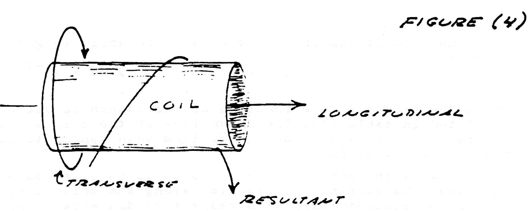
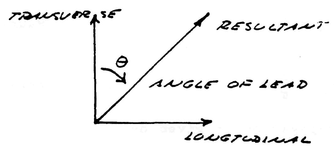
Hence, two distinct forms of energy flow are present in the coiled conductor, propagating at right angles with respect to each other, as shown in fig. 4. Hereby a resultant wave is produced which propagates around the coil in a helical fashion, leading the transverse wave between the conductors. Thus the oscillating coil posses a complex wavelength which is shorter than the wave­length of the coiled conductor.

COIL CALCULATION

If the assumptions are made that an alternating current is applied to one end of the coil, the other end of the coil is open circuited, Additionally external inductance and capacitance must be taken into account, then simple formulae may be derived for a single layer solenoid.

The well known formula for the total inductance of a single layer solenoid is

L=r2N2(9r+10l)

x10-6 Henry (inches) (1)

Where

• r is coil radius
• l is coil length
• N is number of turns

Figure (3)

The capacitance of a single layer solenoid is given by the formula

C=pr	2.54×10-12 Farads (inches) (2)

where the factor p is a function of the length to diameter ratio, tabulated in table (1). The dimensions of the coil are shown in figure (1). The capacitance is minimum when length to diameter ratio is equal to one.

Because the coil is assumed to be in oscillation with a stand­ing wave, the current distribution along the coil is not uniform, but varies sinusoidially with respect to distance along the coil. This alters the results obtained by equation (1), thus for resonance

L0=½L

Henrys (3)

likewise, for capacitance

C0=8πC

Farads (4)

Hereby the velocity of propagation is given by

V0=1L0C0=ηVc

Units/sec (5)

Where

Vc=1με

Inch/sec (6)

That is, the velocity of light, and

V0=ηVc=[1.77p+3.94pn]½

2π109 Inch/sec (7)

Where n = the ratio of coil length to coil diameter. The values of propagation factor η are tabulated in table (2).

Fres=(0.39*ln(h/d)+1.19)*75e6/l

(Hertz)

Thus, the frequency of oscillation or resonance of the coil is given by the relation

F0=V0(l0.4)

Cycles/sec (8)

Where l0 = total length of the coiled conductor in inches.

Figure (4)

The characteristic impedance of the resonant coil is given by

Zc=L0C0

Ohms (9)

Hence,

Zc=NZs

Ohms (10)

Where

Zs=[(182.9+406.4n)p]½

π2103 Ohms (inches) (11)

and N = number of turns. The values of sheet impedance, Zs, are tabulated in table (3).

The time constant of the coil, that is, the rate of energy dissipation due to coil resistance is given by the approximate formula

u=R02L0=(2.72r+2.13l)πF0

Nepers/sec (inches) (12)

Where

• r = coil radius
• l = coil length

In general, the dissipation of the coil’s oscillating energy by conductor resistance:

1. Decreases with increase of coil diameter, d;
2. Decreases with increase of coil length, l, rapidly when the ratio, n, of length to diameter is small with little decrease beyond n equal to unity;
3. Is minimum when the ratio of wire diameter to coil pitch is 60%.

By examination of the attached tables, (1), (2) & (3), it is seen that the long coils of popular designs do not result in optimum performance. In general, coils should be short and wide, and not longer than n=1. The frequency is usually given as F0=Vc/λ0 which by equation (7) is incorrect. Winding on solid or continuous formers rather than spaced slender rods, as shown in figure (1), greatly retards wave propagation as indicated in equation (6), thereby seriously distorting the wave. The dielectric constant of the coil,ε , should be as close to unity as is physically possible to insure high efficiency of transformation.

The equations for the voltampere relations of the oscillating coil are

E.1=j(ZcY0+δ)E.0

Complex Input Voltage (13)

I.1=j(YcZ0+δ)I.0

Complex Input Current (14)

Z1=ZcY0+δYcZ0+δZ0

Input Impedance, Ohms (15)

Where

• E.0= Voltage on elevated terminal
• I.0= Current into elevated terminal
• Yc=Zc-1
• Z0= Terminal impedance
• Y0= Terminal admittance
• δ=u2F0= Decrement
• j= root of -1

For negligible losses and absolute values

E1=(Zc2πF0C0)E0

Volts (16)

I1=(Yc/2πF0C0)I0

Amperes (17)

Where

• C0= Terminal capacitance

By the law of conservation of energy

E1I1=E0I0

Volt-Amperes (18)

If the terminal capacitance is small then the approximate input/ output relations of the Tesla coil are given by

E0=ZcI1

Output Volts (19)

I1=E0Yc

Input Amperes (20)

I0=YcE1

Output Amperes (21)

E1=I0Zc

Input Volts (22)

---

TABLE (1) Coil Capacitance Factor

Length/Width = n	Factor P	Length/Width = n	Factor P
0.10	0.96	0.80	0.46
0.15	0.79	0.90	0.46
0.20	0.70	1.00	0.46
0.25	0.64	1.5	0.47
0.30	0.60	2.0	0.50
0.35	0.57	2.5	0.56
0.40	0.54	3.0	0.61
0.45	0.52	3.5	0.67
0.50	0.50	4.0	0.72
0.60	0.48	4.5	0.77
0.70	0.47	5.0	0.81

TABLE (2)

Length/Width = n	V0 Inches/Sec	Percent Luminal Velocity = η
0.10	9.42 x 10^9	79.8%
0.15	10.9	92.2
0.20	12.0	102
0.25	13.0	110
0.30	13.9	118
0.35	14.8	125
0.40	15.6	132
0.45	16.4	139
0.50	17.2	146
0.60	18.4	156
0.70	19.5	165
0.80	20.5	176
0.90	21.4	181
1.00	22.1	187
1.5	25.4	215
2.0	27.6	234
2.5	28.7	243
3.0	29.7	251
3.5	30.3	257
4.0	30.9	262
4.5	31.6	268
5.0	32.4	274
6.0	33.0	279
7.0	33.9	287

TABLE (3)

L/W =n	Zs
0.10	0.107 x 10
0.15	0.070
0.20	0.116
0.25	0.116
0.30	0.116
0.35	0.115
0.40	0.115
0.45	0.114
0.50	0.113
0.60	0.110
0.70	0.106
0.80	0.103
0.90	0.099
1.00	0.095
1.5	0.081
2.0	0.070
2.5	0.061
3.0	0.054
3.5	0.048
4.0	0.044
4.5	0.040
5.0	0.037
6.0	0.032
7.0	0.028

Electrical Oscillations in Induction Coils:

The following quote is from John M. Miller in Further Discussion on Electrical Oscillations in Antennaes and Induction Coils

“When applying the theory of uniform lines to coils I think a very large error is made at once, which vitiates, very largely any conclusions reached .The L and C of the coil, per centimeter length, are by no means uniform, a neccessary condition in the theory of uniform lines; in a long solenoid the L per centimeter near the center of the coil is nearly twice as great as the L per centimeter at the ends, a fact which follows from elementary theory, and one which has been verified in our laboratory by measuring the wave length of a high frequency wave traveling along such a solenoid. The wave length is much shorter in the center in the center of the coil than it is near the ends. What the capacity per centimeter of a solenoid is has never been measured, I think, but it is undoubtedly greater in the center of the coil than near the ends.”

 

Request to find by Eric: Abnormal Voltages In Transformers. J.M. Weed. American Institute of Electrical Engineers. September 1915, p 2157

The following is from the Steinmetz book Theory and Calculation of Transient Electrical Phenomena.

 

 

In response to: source

The fence is a single turn primary and a 22 turn secondary. Primary and secondary windings have the same weight. The size of wire used in both is 8 gauge. Obviously paralleled in the primary into one large conductor. The extra coil is wound with #10 wire. More specifically equal width to height ratio and the extra spacing on the outer turns is due to the accelerated voltage gradient. All of your odd harmonics add up at this point, and produce an enormous rise in electrostatic potential.

 

---

DE N6KPH