
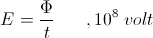
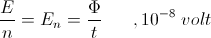
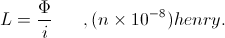
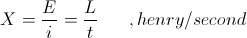
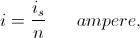
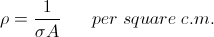
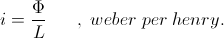
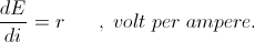
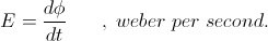
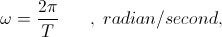
(1) Electro-Motive Force, or E.M.F., is a consequence of the law of electromagnetic induction, Faraday’s Law. This is his Electro-Tonic State. It is dimensionally the time rate at which magnetic induction is produced or consumed, or in other words “moved about”. The dimensional relation is given asWeber per Second,This defines E.M.F. in Volts.
(2) The notion exists that the electro-motive force, E.M.F. in volts, is established by “cutting” lines of magnetic induction via a so called electric conductor. This “cutting” is then said to impel the motions of so called electrons within the conducting material. It is however that a perfect conductor cannot “cut” thru lines of induction, or flux lines, Phi. Heaviside points out that the perfect conductor is a perfect obstructor and magnetic induction cannot gain entry into the so called conducting material. So where is the current, how then does an E.M.F. come about? Now enters the complication; it can be inferred that an electrical generator that is wound with perfect conducting material cannot produce an E.M.F. No lines of flux can be cut and the aether gets wound up in a knot. Heaviside remarks that the practitioners of His Day “do a good deal of churning up the aether in their dynamos”.
(3) A good analogy exists between the induction generator, and its hydraulic counterpart, the centrifugal pump. The pump casing is filled with water in order to operate. Once filled with water, in the condition that the suction and discharge valves are shut thereby confining water to the pump casing, the pump consumes no energy from its shaft. The pump impeller rotates with no damaging pressure, and the water and impeller rotate in step within the pump casing. Upon opening the valves the shaft is loaded by the energy required to move the water thru the pump casing. The law of energy continuity is established in that the energy consumed by the pump shaft is continued as the energy delivered to the motion of the water. Also by the law of reciprocity the energy can be extracted from the flow of water and continued as the delivery of energy to the shaft. Now the centrifugal pump is a centrifugal turbine.
In this configuration the centrifugal apparatus is connected with an electro-dynamic machine, this an induction motor. This induction motor delivers motive energy to the centrifugal pump. It is however that the centrifugal apparatus is also capable of serving as a centrifugal turbine delivering energy to the motor shaft and hence now this induction machine is and induction generator. Again the law of energy continuity is established in that the motive energy taken from the flow of water is delivered to the shaft of the induction machine. The law of reciprocity is established in that the energy continuity is equivalent in both directions of power flow. (This is not possible with an engine)
(4) The induction machine is in some ways analogous to the centrifugal machine. In order for the centrifugal machine to function the casing must be filled with water. Likewise, the induction machine must be filled with magnetism, this in order to function as a generator or motor, otherwise the shaft & rotor spin free transferring no energy. This describes the torque converter in an automatic transmission, a fluidic clutch. As with the centrifugal machine, once it is filled with magnetism, it is that no load appears on the shaft of the induction machine when its circuit breaker is open. Only upon closing the breaker can energy be supplied to the shaft as an induction generator, or taken from the shaft as an induction motor. This analogy between the centrifugal machine and the induction machine fails in one aspect, where the body of water in the casing is moved along with the flow, the magnetism in the induction machine remains stationary and static. No magnetic energy is required beyond that necessary to fill the induction machine. Hence this magnetizing force can be maintained by an electro-static condenser.
It is however that a large electro-magnetic energy is developed by the induction generator, taking this from the rotor shaft and its prime mover. Here the magnetic induction & E.M.F. developed greatly exceeds that involved in the excitation of the induction machine. This opens the question as to where exactly does this generated electricity come from, and likewise with an induction motor where does the consumed electricity go. A sea of partial differential equations is of no assistance in finding the answer. It is occult to human kind, and the actual dimensions of electricity remain unknown. Here is where we begin.
BREAK DE N6KPH
(3) During the dark ages the U.S. Navy became increasing disillusioned with the wireless developments provided to them. Poor and unreliable performance along with the dependence upon civilian technicians frustrated the efforts of establishing a reliable and effective naval radio communication system. The Alexanderson system along with later developments by Edwin Howard Armstrong would mark the end of the radio dark ages. The U.S.Navy was quick to co-opt the Alexanderson system into its communication network. KET and WII were its first Alexanderson stations for V.L.F. transmission. The Navy froze all radio patents from the dark ages, ending the relentless patent wars. The assistant secretary of the Navy Franklin D. Roosevelt used this opportunity to outlaw radio for civilian use, ending the radio experimenter. Under the direction of Admiral Bullard, U.S.N. A “Radio Corporation” was organized to serve as a holding company for radio patents and developments. Hence the birth of R.C.A. in 1919, and also the birth of radio as it has become known. The year 1919 begins the age of electromagnetic radio and its domination of transmission theory. But today we are interested in the unknown radio of yesterday, that before 1919, that of Tesla and Alexanderson.
(4) The development of the thermionic vacuum tube by General Electric and Bell Telephone put this device in the forefront of radio advancements. This could never happen in the hands of the inventor, Lee DeForest, so he was bought out by A.T.T. And his patents placed into the patent pool of the Radio Corporation, developing into a monopolistic trust. The efforts of Edwin H. Armstrong for R.C.A. and Langmir for G.E. Led to the Pliotron Power Oscillator utilizing the UV-207 thermionic, water cooled, vacuum triode. This instantly obsoleted use of the Alexanderson alternator for the production of large quantities of radio frequency power. His system became obsolete almost as soon as it was installed (1921), R.C.A. Radio Central, Rocky Point, NY. Thus the Alexanderson system became a dinosaur, to be buried and then forgotten. In the American tradition it was all smashed into rubble and then thrown over the cliffs into the sea. (Bolinas). Another historic “elimination”.
(5) Becoming obsolete, the Alexanderson system was regarded as of no significance to the “modern understanding” of electricity. As electronic ideas began to overtake electrical ideas a misunderstanding developed with regard to the electric wireless of Tesla and Alexanderson. Radio became married to electro-magnetism, and electricity became married to the electron. It is however that the Alexanderson system is electrical, not electronic. It was in fact developed specifically to avoid the electronic patents, and also work in a way not already specified in the patents of Nikola Tesla. The magnetic amplifier served as a kind of magnetic transistor, eliminating the need for the electronic vacuum triode of DeForest. The Alexanderson aerial is unlike the structures of Tesla and Marconi and also is not an electro-magnetic radiator. The developments of Ernst Alexanderson operate in a unique fasion, unlike more commonly known electrical developments. Hence the importance of the study of the elements of the Alexanderson system.
(6) The Alexanderson system consists of three principle elements;
I) The Variable Reluctance Alternator, for the generation of V.L.F. Power.
II) The Magnetic Amplifier, for the modulation of this V.L.F. Power.
III) The Multiple Loaded Aerial, for the transmission of the modulated V.L.F. Power.
All three of these elements are based upon radical departures from more conventional electrical designs. The Law of Electromagnetic Induction finds a new meaning in these particular developments of Alexanderson. These represent a “third way” in the development of electromotive force. It can be expected that certain anomalies as well as certain oppositions by “the group” in the Law of Energy Continuity are to be found in the elements that comprise the Alexanderson system. Such is demonstrated with the Variable Reluctance Generator seen in the Borderland video, this machine similar to the Alexanderson alternator in principle.
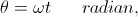
(7) Electro-Motive Force is brought about by magnetism in motion. The motional relationship between magnetism and its bounding metallic-dielectric geometry give rise to E.M.F., this E.M.F. as a reaction to magnetic motion is and inertial force, at least as it is commonly understood. The production or consumption of electro-motive force is developed by three distinct relations;
I) The E.M.F. of Variable Magnetic Induction, such as with the static transformer,
II) The E.M.F. of Motional Magnetic Induction, such as with the rotating motor-generator,
III) The E.M.F. of Variable Magnetic Inductivity, such as the static magnetic amplifier, or rotating variable reluctance alternator.
In basic terminology, with the static transformer it is the intensity of the magnetism is variable, in the motor-generator the position of the magnetism is variable, and in the magamp or Alexanderson alternator it is the containment of the magnetism is variable.
In the static transformer the magnetizing force is made to vary, as with alternating current. This gives rise to a continuously variable quantity of magnetic induction developing a continuously variable E.M.F. Induction is the variable.
In the motor-generator the position of the magnetic induction is made to vary via rotation. This rotation is constant developing an E.M.F. which is also constant and constantly rotating as is the magnetism. Here the E.M.F. is not alternating as with the static transformer, but has a vector of constant length in constant rotation. Hence this E.M.F. is in a polyphase or direct current relation. Orientation in Space is the variable.
In the magnetic amplifier, or Alexanderson alternator, the inductivity of the medium supporting the magnetic induction is made to vary, this by saturation or relative motion. Hereby magnetism is made to enter or leave the magnetic medium thru the variation of the storage capability of that medium. The E.M.F. developed is in order to facilitate the flow of magnetic energy into, or out of, the medium of variable magnetic inductivity. Storage Capability is the variable. This is the “third way”.
BREAK DE N6KPH
Law of Electro-Magnetic Induction, Three (1 of 2):
(1) The analysis of the Faraday Law, the Law of Electro-Magnetic Induction, continues here with the “Theory and Calculation of Alternating Current Phenomena”, by Charles Proteus Steinmetz, PhD, 1916. This is the fifth edition, which is partitioned into several other allied books. Two chapters are used in the analysis here, chapter three, “The Law of Electro-Magnetic Induction”, and chapter twenty-five, “Distortion of Wave-shape and Its Cause”. The chapter on reaction machines is missing from the fifth edition as it is partitioned into an allied volume. The 1900 edition is more suited for the study of Synchronous Parameter Variation in terms of a wider conception, however the 1916 edition is sufficient for the analysis here, this is all glom provides.(2) Many of the expressions given by Steinmetz are unclear, particularly the harmonic expression of the reactance variation. The signs and symbols in the subscript have misprints, and the dimensions often do not line up. It must also be remembered that Steinmetz was forced to alter his mathematical expressions by the P.E.E.E. He literally came under attack by the pendants particularly for his development of the “Law of Hysteresis”. Hence Steinmetz changed his expressions because of PEEE adopted international standards, to quote;
“Thus for the engineer familiar with one representation only, but less familiar with the other, the most convenient way when meeting with a treatise is in, to him, unfamiliar representation is to consider all the diagrams clockwise and all the signs of j reversed.”
“In conformity with the recommendation of the Turin Congress – however ill conceived this may appear to many engineers – in the following the Crank Diagram will be used, and where ever conditions require the Time Diagram, the latter be translated into the Time Diagram.”
In basic terms if it seems daylight savings time is a bad idea, now it is a standard that all clocks must turn backwards in their rotation.
(3)Steinmetz does not use rational units in the development of his expressions. Heaviside warns that this is fatal to a solid theoretical understanding. The result is a quagmire of four-pi, one over c square, one over ten and all multiplied by ten to the eighth power. Steinmetz compounds the confusion by using cyclic frequencies in cycles per second rather than angular frequencies in radians per second. This results in the continual appearance of two-pi in all his expressions. The numeric pi is seen to appear and vanish so many times in Steinmetz equations and formulae that its meaning has become lost.
Steinmetz works backward from the practitioner’s law for the output of a D.C. dynamo,

Where E is the developed E.M.F., F is the frequency in cycles per second, n is the number of turns, and phi is the quantity of magnetism. The numeric 4 is the number of inductions per cycle, one for each angular quadrant. Steinmetz considers this as an average E.M.F. where in actuality the average value of a sine wave is zero. His average value is the rectified value, that of a half wave. This in order to express the E.M.F. in maximum or peak values, the factor pi over two must be affixed to the average E.M.F. This creates another pi in all the expressions, fading in and out like a ghost thruout.
In the development of his expressions, by working backwards, it appears to be a “force-fit” in order to arrive at an already predetermined result, a form of contrivance to quickly reach a practical result. This obviates any understanding of the theoretical conditions involved. Steinmetz created his system of mathematics for the practicing engineer, not the theoretician. This riles the pendant, nemesis ensues.
(4) As is well known Steinmetz introduced many mathematical concepts to greatly simplify the understanding and utilization of alternating current electricity. But General Electric did not want him to put too much know how in his books. Other than Steinmetz, it was only Nikola Tesla of Westinghouse Electric that could make working A.C. equipment. But Tesla did not write books, his failing, out loss.
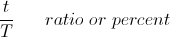
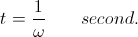
Thruout his writings Steinmetz utilizes a dimensionless time operator which greatly simplifies the expression of alternating current phenomena. An angular rate is substituted for a time rate. It is an instantaneous position variable along the A.C. cycle, the dimension of time is canceled by the angular frequency in radians per time, given is,
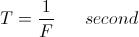
t = Time Variable, second
T = Time Period, second
F = Frequency, cycle per second
 = Time Rate, per second
Hence the following expressions,

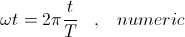

Where the factor 2pi can be called an “angular tensor”.
The differential expressions for alternating current phenomena become a dimensionless operator, not a time rate

is now,
Now it is a variation in angular position, radians are dimensionless.

Hence for 60 cycles the angular position is given by
For one radian it is that

This the time taken for the 60 cycle A.C. wave to advance one radian in its angular progress thru a cycle. This is a dimensionless operation. This angular position variable is like an instantaneous versor operator of infinitesimal unit positions. This operator is then compounded with the quadrantal A.C. operator,

Where  is given by

The result is the segregation of the resistive from reactive terms, or more properly the kilowatts from the kilovolt-amperes reactive. Great simplification is derived here thru inductance expressed in ohms as is resistance, and by capacitance expressed in siemens as in conductance. The differential expressions vanish and Ohm’s Law as well as Kirchoff’s Law can be utilized in alternating current circuits. This is known as the “Steinmetz Method” a mathematical breakthru for the expression of the phenomena of alternating electric waves. This was the birth of electrical engineering in alternating current systems. While the engineer loves it, (This is why E.F.W. Alexanderson came to America, in order to work with the great engineering mathematician, Dr. Steinmetz.) the pendant has a deep contempt for the Steinmetz methodology (Pupin). At a common level, upon my unusually high test scores in naval electronics entry school, this thru my use of the Steinmetz method, naval instructors accused me of cheating, and caused me trouble!
BK DE N6KPH
Law of Electro-Magnetic Induction, Four:
And,

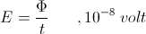
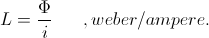
The volt-second defines the unit of “magnetic charge”, just as the ampere-second defines the unit of “electric charge”. Hence, and E.M.F. of one volt, over a duration of one second, produces or consumes one unit of magnetic induction, this induction consisting of 100 million lines of magnetic flux. One flux line, or tube of induction, can be taken as a discrete entity, and of a distinct dimensional size, this a numerical constant. In other words a quantum size of magnetic induction defines all lines of induction as being the same size. It is then that this line of induction is a constituent of the Planck, a quantum dimensional relation consisting in part of a quantum of magnetic induction. The factor of ten to the eighth power partially defines the size of the Planck, in defining a distinct line of magnetic induction. Here is a partial answer to the old question of “how big is a Planck?”
(2) The volt-second, or magnetic “charge” is the conjugate of the ampere-second, or dielectric charge. Magnetic charge is in weber, dielectric charge is in coulomb, this dimensionally given as


In common practice the unit of dielectric charge is the ampere-hour, and defines the quantity of electricity into, or out of, an electric accumulator (storage battery).
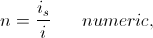
Considering the ampere-second it is when the displacement current, I, in amperes, passes thru an impedance, Z, in ohm, that energy is exchanged with the dielectric field of induction. In this passage the displacement current, I, in amperes is transformed into a magneto-motive force, i, also in amperes. This i relates to the metallic, and the displacement I relates to the dielectric. When this impedance, Z, consists of a resistance, R, in ohm, the displacement current gives rise to an electronic current, i, this also in amperes, the energy in the dielectric is dissipated at the rate,

(3) The concept of the accumulation of “charge” is normally not considered when dealing with a magnetic field and the energy it contains. This magnetic “charge” is analogous to the dielectric charge. Magnetic charge is given as the volt-second, this a volt of E.M.F. When this volt of E.M.F. is impressed upon an admittance, Y, in siemens, that energy is exchanged with the magnetic field of induction. Hereby the E.M.F., E, in volt, is transformed into an electro-static potential, e, also in volt. When this electro-static potential is impressed upon a conductance, G, in siemens, this conductance dissipates the energy stored in the magnetic field of induction at the rate,

It was shown in the “Four Quadrant Theory”, E.P. Dollard, that dielectric discharges give rise to strong currents, whereas magnetic discharges give rise to high E.M.F.s. This was shown in recent experiments with the 60KV, 3000KVA, power line transformer. The magnetic charge drawn from only a 12 volt car battery can have destructive consequences if discharged rapidly by an open circuit, hence the flashover on the bushing safety gap.
(4) Electro-motive force is the medium by which energy is supplied to, or demanded of, the magnetic field developing this E.M.F. When this E.M.F. is made to be an electro-static potential, then energy can be exchanged. Part of this energy is stored, thru a displacement current,

or it is dissipated,
or combined, for an A.C. wave,

Gives the total electrical activity of the magnetic field of induction in the exchange of its energy to an external form. In this relation the E.M.F., E, is made equivalent to electro-static potential, e, this via a parallel connection of the magnetic inductance to the external system. Conversely, for the dielectric field, the displacement current, I, is made equivalent to M.M.F., or electronic current, i, this via a series connection of the dielectric capacity to the external system. Hence the Law of Electro-Magnetic Induction is entirely analogous to the Law of Dielectric Induction, and the understanding of one can be derived from the other.
BK DE N6KPH
The Law of Electro-Magnetic Induction, Part 5. (1 of 2):
And by algebraic operation, the magnetic “charge” is,
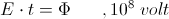
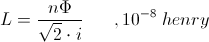
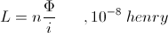
The Time Interval, t, is one second, and the quantity of induction,  , is one hundred mega-lines of flux. This relation defines one volt of electro-motive force. In the next paragraph, page 16, Steinmetz turns the eighth power around, this to the negative eight, altering the relation to,
Compounded on this relation is the number of turns in the coiled winding,
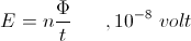
And hereby it is,
Where En is the volt per turn and n is the number of turns. No explanation is provided as to the reason for the reversal of the power of ten, from plus eight, to minus eight. We are off to a good start here!
The number of turns in the winding act co-jointly to multiply the E.M.F. These turns also act co-jointly to the multiply the current. This current, i, in amperes, is continuous throughout the coiled winding. As each turn comes about it carries current, i, with it, round and round again, throughout the total number of turns. The net result is a sheet current, this consisting of n individual currents. This is given by the relation,

This sheet current is the magneto-motive force that maintains the magnetic induction. This is in distinction to the current, i, which is related to the “electronic” current. Hence the M.M.F. is expressed in ampere-turns, the “electronic” current, i, and the number of turns, n. For example, a reactance coil has 1000 turns, and it is drawing a current, i, of one ampere, the sheet current of the coil, is, is now 1000 amperes. Hence this coil is operating with a M.M.F. of 1000 ampere-turns. Large M.M.F.’s can be produced with small currents thru the compounding of these currents via multiple turn windings of many turns. The limiting factor is the accumulation of series resistance as the winding gets longer in length.
This was an important discovery in electro-magnetism. It’s first engineering application was the Morse Telegraph Coil as developed by Joseph Henry, the American Faraday.
(2) These multiple turns not only multiply the current, i, they also multiply the E.M.F., E. The currents compound, side by side, in a parallel fashion, this creating a sheet current. The E.M.F. per turn compounds, end to end, in a series fashion. Each and every turn develops an identical E.M.F. All turns are linked together thru the mutual magnetic induction which surrounds the entire winding. Each individual E.M.F. adds to the next, in a series manner, developing a total E.M.F., that of the entire winding.
This is expressed in the relation,

Where,
Eo, the total end to end E.M.F.
E, the individual turn E.M.F.
For example, the same reactance coil, 1000 turns. This coil is discharged at a constant rate over a period of one second. During this discharge each turn develops an E.M.F. of one volt. The coil has 1000 turns, hence the total E.M.F. at the ends of the windings is 1000 volts. This is the principle of automobile ignition coil, a magnetic discharge device.
Here established is two relations, one for the total M.M.F.,
The other for the total E.M.F.,
The individual currents are identical thruout the coiled winding, no gradient exists in this current. The individual E.M.F’s are also identical, but not as with the current. A gradient exists in between the turns as the E.M.F. compounds along the winding. Hence a voltage gradient exists along the winding length expressed as volts per turn. Here in this metallic-dielectric geometry the magnetic force and the dielectric force are oriented in the same direction, (MK).
The Law of Electro-Magnetic Induction, Part 5. (2 of 2):

Where,
F, frequency in cycles/second.
Steinmetz states here the numeric four results from the lines of force being “cut” four times in one complete rotation or cycle of alternation. This gives rise to four quarter wave surges of induced E.M.F. Each is in succession, one follows the other. These surges alternate in half wave sets, first plus-minus, then minus plus. For example, consider the 1000 turn reactance coil. At the onset of the cycle the magnetic induction expands outward, this with a “north” polarity. As it expands it must force its way thru the windings, giving rise to an E.M.F. in a reverse direction. As the cycle progresses the magnetism expands to its maximum extent and then is withdrawn, back inside the coil. This back surge of magnetism must again force its way thru the windings, giving rise to an induced E.M.F. in a forward direction. The first half cycle is now complete, giving a reverse and then a forward induced electro-motive force. At the onset of the next half cycle the magnetic induction expands outward again, this time it is of a “south” polarity. As it expands it again forces its way thru the windings giving rise to an induced E.M.F. in the forward direction, forward because the magnetism is now “south” rather than “north”. As this next half cycle progresses the magnetism expands to its maximum extent and is withdrawn. This back surge of magnetism must again force its way thru the windings to get back inside. This gives rise to an induced E.M.F. in the reverse direction and then the cycle is complete. Hence the existance of four distinct E.M.F. each existing in one quadrant of the A.C. cycle.
1) Expansion, north (+).
2) Contraction, north (-).
3) Expansion, south (-).
4) Contraction, south (+).
Euro-standards require reverse to be positive, its the law, the law of the crank. Reverse means here a back E.M.F. in opposition.
It should be noted that if the windings are shorted with no resistance, it is that no E.M.F. can exist and thus no motion of the magnetic induction is possible. This will halt the rotation of the dynamo.
(4) Steinmetz continues with the development of the dynamo formula. The maximum, or peak, value of E.M.F. is given by the relation,
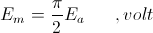
This alters the dynamo formula into,

Here it is given that,

Steinmetz fails to incorporate this angular velocity or frequency, into his equations. This would simplify the dynamo equation to,

or on a Per Turn Basis,
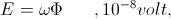
Substituting the relation
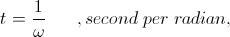
The dynamo formula now becomes the basic expression of the law of E.M. Induction, this given as,
This on a per turn, or unit, E.M.F. basis. Hence a volt is given as weber per second. The radian is dimensionless.
Thruout his writings it is that Steinmetz refuses to use the angular frequency,  , and insists upon the use of the cyclic frequency, F, cycles rather than radians. This unnatural form of expression results in the continued appearance of the factor two pi thruout his equations. This makes each equation that much more complex and gives rise to the situation of interferences with other pi factors causing cancellations and squares.
Steinmetz continues here to give the relation for the effective value of E.M.F.,
This is also known as the root mean square value, (RMS).
The dynamo formula now take the form,

This is the “Steinmetz Formula” for the law of E.M. Induction, a convoluted mess! This is a “practitioner’s” formula for winding dynamo coils, not a starting point for a theoretical study of A.C. phenomena.
BK DE N6KPH
Reference:
“Intro to E.M. Theory”, Vol I by Oliver Heaviside, note “Practitioner”.
(1) Steinmetz closes chapter three in his A.C. book, 1916 edition, with his development of the concept of Inductance. Here given, for the first time in chapter three, is the current, i, in ampere. It is the “electronic” current, for the lack of a better term. Steinmetz gives the relation,
This is the Magnetic Inductance, also known as the co-efficient of magnetic energy storage.
Steinmetz complicates this relation by giving the current, i, in effective values, an unnatural form. The relation is given by,
Hence the resulting expression is given by,

Transposing his relation gives,
This derives from Steinmetz’s expression the co-efficient of self induction.
Using maximum rather than effective values for current simplifies the relation to,
This the basic expression for the co-efficient of self induction.
(2) This self induction is a non motional, or static, induction. This represents the reactance coil. It is important to notice that the self induction is distinct from the motional induction produced by the dynamo. The motional relation, that of rotary motion, is given by the relation,

The induction for the static, or stationary, condition is given by the relation,
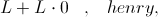
In the static expression the number of turns, n, and the factor of ten to the minus eighth, are absorbed into the henry, that is,
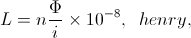
becomes
(3) Continuing in chapter three Steinmetz introduces the concept of Reactance. The relation is given by,
Substituting the relation,

Establishes the basic Ohm’s Law expression for alternating currents,
X is called the reactance of the coiled winding. Transposing gives the expression for the reactance as,
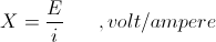
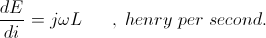
And it is that volt per ampere defines the dimensions of the ohm. This volt per ampere can also be expressed as a henry per second, giving the relations,
And it is,
This expression of reactance can be considered a synchronous inductance, this in an A.C. circuit.
(4) The total magnetic induction can be sub-divided into a pair of independent factors.
One, the intensity of the magneto-motive motive force, this maintaining the quantity of magnetism, Force, i, in ampere.
Two, the concentration , or inductance, containing the quantity of magnetism, Concentration, L, in henry.
These two factors are related thru the Law of Magnetic Proportion, given by,
Where, i, is the ampere of current. Transposing gives the relation for magnetic induction as,

Hence the total magnetic induction is the product of two Independant Parameters, each of which contributes to the induction. Each of these two parameters can be variedseparately. The E.M.F. is developed thru the resulting variation of the total magnetic induction.
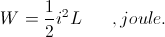
The total energy contained in the magnetic induction is given by the relation,

It was given that,

Substituting this into weber-ampere gives,

And this leads to the expression of magnetic energy as,
(5) The quantity of magnetic induction is made to vary by variation of the current or the variation of inductance, or by the variation of both. This variation of magnetism that results from the parameter variation gives rise to a variation of the quantity of stored energy contained in the magnetic induction. The E.M.F. developed by the variation of magnetism is the means by which the stored energy can either leave or enter its magnetic form. It is then the current, or M.M.F., represents the potential energy stored in the magnetic field, and the E.M.F. represents the kinetic energy given or taken by the magnetic field.
This is analogous to the dielectric field. Here it is the electro-static potential, e, in volt that represents the potential energy of the field. The displacement current, I, in ampere then represents the kinetic energy taken or given to the dielectric field. Hence,
Therefore where it is that the voltage, e, is the electro-static potential, it is the M.M.F. (and its current, i,) is the magneto-static potential.
Both potentials in themselves do not represent energy, only the force required to maintain this energy in a static, or potential, state.
(6) The M.M.F. is the force holding the magnetism in place. A stationary magnetic field needs a continuous current to remain stationary.
The inductance is the holder of the magnetism. An invariant inductance can hold a stationary magnetic field of induction in place.
Variation of either the M.M.F. or the inductance requires the magnetism move. This gives rise to an E.M.F. of energy transfer, this as a result of a time rate of change in the quantity of magnetism. The E.M.F. is directly proportional to this change, the quicker the change, the larger the E.M.F.
Neither the M.M.F., nor the inductance, represent energy. They are only factors of the induction, parts of a whole. While each parameter effects the magnetism as a whole, the effects of each are not interchangeable, and this needs to be taken into account regarding the Law of Energy Continuity.
(7) In the static reactance coil it is the intensity of force, as a current, that is made to vary. This variation is expressed in ampere per second,

Where,

The inductance of the reactance coil is constant, or invariant in this situation. Hence the E.M.F. developed by the reactance coil is derived from the time rate of current variation only. This is expressed by the relation,

Where,  , ampere-second. It is customary however to express this relation using

and
But here in the reactance coil the inductance is in-variant, no such henry per second exists. It is the ampere per second which acts here. Hence in its common expression the term reactance can be misleading.
The Law of E.M. Induction, Part 6 (3 of 3):
(9) Parameter Variation of the inductance is expressed by the relation,

And here it is

In comparison, for the condition of parameter variation of the current the relation is,

And here it is given,

Hence,
Current variation in ampere per second, , and inductance variation in henry per second, XL, two distinct variations.
In these two distinctly different conditions, each have the same component dimensions,

These three dimensional relations engender but one magnetic field. However the order in which these three dimensions are situated gives rise to two distinctly different conditions, that is,
Ampere – Henry per Second,
Henry – Ampere per Second.
The Law of E.M. Induction exists in two forms with the same basic dimensions. Hence the term reactance can take on two new meanings, the reactance of self inductance, and the reactance of inductance variation,


Only in the variant inductance are the dimensions correctly in the henry per second.
(10) For the condition of current variation with respect to time the inductance is a constant, or invariant. The alternating E.M.F. is produced by a current alternating between maximum values of opposite polarity, positive and negative. A zero crossing results, between maximum values.
For the condition of inductance variation with respect to time the current can be constant, a direct current, that is, invariant. The alternaing E.M.F. is produced by the pulsation of inductance between maximum and minimum values. There is no zero inductance. Both the maximum and minimum values are positive.
Where it is possible to reverse the current, or make it pulsating, the inductance cannot be reversed. Negative inductance is undefined. The inductance variation is intrinsically asymmetrical in nature. The variation exists as a percentage of modulation, 100 percent being variation of inductance between zero inductance, and the maximum inductance, values, as limits.
(11) This parameter variation can be extended to both the current and the inductance, both in variation together. Each can be in variation at their own time rates, each at its own frequency and phase angle. This gives rise to a complex E.M.F. containing modulation products of sum and difference frequencies, with the originating frequencies suppressed. This is known as a double sideband modulation. The E.M.F. is of the form,

Here enters chapter 25, of Steinmetz’s A.C. book, 1916 edition. The chapter is titled “Distortion of Waveshape and Its Cause”. Here Steinmetz develops expressions for what is called Synchronous Parameter Variation, for both rotating and static apparatus. This serves as an extension on the Theory and Laws of Hysteresis.
BK DE N6KPH
Law of Electro-Magnetic Induction, Seven (1 of 3):
One, the Magneto-Motive Force, is, in Ampere-Turn,
Two, The Magnetic Inductance, L, in Henry.
Variation of one or both of these factors results in the variation of the quantity of magnetism. In turn this variation in magnetism develops and E.M.F. in direct proportion to the time rate of this variation. This E.M.F. is developed thru Parameter Variation.
Variation of the parameter magneto-motive force is brought about by the variation of the current, i, in ampere which produces this M.M.F. The M.M.F. and its current are related by,
Or,
Where
n = Number of Turns.
This number, n, is the ratio of M.M.F. to its current, and it serves as a magnification factor for current flow.
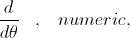
Variation of the parameter Inductance is brought about by the variation of the factor
Where
 is the magnetic permeability, in centimeter
 is the magnetic path length, in centimeter.
This factor,  , is the effective permeability of the magnetic circuit. The magnetic permeability is a characteristic of the medium which supports the magnetic induction. This is not to be confused with the relative permeability. The magnetic permeability
, centimeter
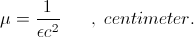
is an Aether constant derived from One Over c Square. The relation is given by,

Where

c is the Velocity of Light.
Hence the relation is given as
This is the magnetic permeability. In order to simplify mathematical expression the relative permeability is often used. It is given by the relation

Where
 is the magnetic permeability of free space or the Aether. Here then exists three expressions for permeability;
One, Magnetic Permeability,
, Centimeter,
Two, Effective Permeability,
, Numeric,
Three, Relative Permeability,
 , Numeric.

Where
A is the sectional area of the magnetic induction, in centimeter square
 is the total flux inter-linkages between the current, i, and the magnetic induction,
  .
.
is the effective permeability, a numeric.
For a unit turn the relation becomes,

The relation hereby derived is given as,
This parameter,
 , is called the Reluctance of the magnetic circuit. This reluctance is a mathematical fiction given to give an analogy between the magnetic circuit, and the electric circuit. Where it is resistance in an electric circuit, it is a reluctance in a magnetic circuit. Reluctance is hereby a magnetic resistance. This analogy does not recommend itself. It has become commonplace to express parameter variation in terms of Variable Reluctance. Such is the “Variable Reluctance Generator”. The factor, , the effective permeability is more suited for the expression of parameter variation.
The two basic expressions for Magnetic Parameter Variation are thus,
The expression of parameter variation of current,
And the expression of parameter variation of Inductance,
(3) The Magnetic Inductance is formed from several factors, or sub-parameters,
n, Number of Turns,
A, Sectional Area,
, Path Length,
, Magnetic Permeability.
The number of turns, and the sectional area are in general invariant. The number of turns is fixed by the impedance, and the sectional area is fixed by the volt-ampere capacity. The path length can be variable by mechanical means. The magnetic permeability can be made variable by magnetic means.
The path length and the magnetic permeability are directly related as they have the same dimension, centimeter. They are both lengths, and their ratio is the effective permeability. This is the parameter to undergo variation.
(4) Permeability works thru the dimension of length, here in centimeter. The length of a magnetic flux line determines the amount of M.M.F. required to maintain that length. A force is required to hold this line in place. The more the flux line is stretched out, the greater the M.M.F. required. This determines the magnetic gradient along the flux line as,
The flux lines are elastic, if stretched out, they hold the energy required in this stretching and it returns when the stretching force is withdrawn. During the interval in which the flux line expands or contracts an E.M.F. is developed to facilitate the movement of energy into, or out of, the elastivity of the magnetic flux line.
If now the magnetic permeability is made to increase, the M.M.F., and thus the current, required to maintain a flux line at a certain length is decreased in proportion to the increase in permeability

Hence the magnetic permeability acts to shorten the lines of magnetic induction. This is to say that the magnetic permeability allows the magnetism to contract into it. In a magnetic path of centimeter length, a path of high permeability has a much longer effective path length than that of a low permeability. The relation is given as

is the relative permeability, a numeric proportion. For example, iron has a relative permeability of,
= 1000 numeric.
A portion of this iron is in the magnetic path and the length of this portion of iron is,
= 1 , centimeter
The effective path length along this iron is then given as

If this magnetic permeability undergoes parameter variation, it results in an effective variation in path length, this for the Magnetic Induction.
(5) The effective permeability can be made variable thru mechanical and magnetic means. Variation is produced mechanically by the insertion and removal of permeable material into & out of the path of magnetic induction. This results in the variation of the effective path length, and thus a variation of the effective permeability, .
In many magnetic materials their magnetic permeability is a function of the flux densities within these materials. The greater the flux density, the less the permeability. When the flux density is increased beyond a certain point the magnetic permeability of the material becomes that of free space. This is known as Saturation. Hereby the magnetic permeable material can be made to vary its permeability by the application of a magnetic field of induction. This in turn gives variation to the effective permeability,
, and thus a variation in effective path length.
(6) The general expression for magnetic induction is given by the relation,

In this relation two parameters can be varied. One is the current can be made variable, in turn giving a variation of M.M.F. The other is the effective permeability can be made variable, this in turn giving a variation of inductance. The current, i, and the effective permeability,
, undergo variation and give rise to a variation of Magnetism, . This variation of magnetism develops and E.M.F. Three basic relations exist,
One,
Two,
Three,
These fundamental relations bear resemblance to those of Ohm’s Law, as basic expressions of proportionality.
Relation one expresses a conservation of magnetism, . This gives the Motor-Generator relation. Here an increase in current relates to a decrease in inductance, or an increase in inductance relates to a decrease in current. This proportionality maintains a constant quantity of magnetism.
Relation two expresses a conservation of Current, i. This gives the variable parameter relation. Here an increase in magnetism relates to an increase in inductance, or a decrease in inductance relates to a decrease in magnetism. This proportionality maintains a constant current.
Relation three expresses a conservation of inductance. This gives the reactance coil relation. Here an increase in magnetism relates to an increase in current, or a decrease in current relates to a decrease in magnetism.
In any one of these three various conditions that give rise to a variation in magnetism the E.M.F. which results from this variation transfers energy into, or out of, the Magnetic Field of Induction, . Here derived is a more general expression for the Law of E.M. Induction for the study of parameter variation in electro-magnetic systems.
BK DE N6KPH
. Current, i, and permeability factor, , are the two parameters which can undergo variation in order to give a variation in the quantity of Magnetism, .The condition in which only the current undergoes variation exists with the Reactance Coil. Here the inductance is a constant, it is a factor of proportionality. This is expressed in the relation,
Here a sine wave of current develops a sine wave of magnetism. Both waves exist in a direct proportion, L, and are thus “in phase”.
For the Reactance Coil the Law of Energy Conservation is satisfied. All the energy given to the magnetism is given back by the magnetism, no gain or loss. This movement of energy is facilitated by the induced E.M.F.
The condition in which only the Inductance undergoes the Parameter Variation exists with the Magnetic Amplifier, or the General Parametric Apparatus. Here the current is constant, it is a factor of proportionality. This is expressed by the relation,
Here a sine wave of Inductance Variation develops a sine wave of Magnetism. Both wave exist in direct proportion, i, and thus are in phase. Energy is exchanged thru the developed Induced E.M.F.
Here the Law of Energy Conservation is not satisfied. The Energy given to the Magnetism is not the Energy given back by the Magnetism, there is a gain or loos of Energy. In this situation the Law of Energy Continuity must be considered.
The condition in which the Magnetism is a constant is the Motor-Generator. This is expressed by the relation
Here it is both the Current, i, undergoing variation and the Inductance, L, undergoing variation, these in an Inverse Proportion in order to maintain a constant Magnetism. As sine wave of Inductance gives a sine wave of Current, but here the two waves are in Phase Opposition, that is, “out of phase”.
Because the Magnetism is “Static” no Energy is exchanged. Thus no “Energy Law” is involved in this condition of constant Magnetism. Hereby no E.M.F. is developed, the E.M.F. of the Motor-Generator is derived solely from the Rotation of the machine. The Law of Energy Continuity is involved here in that the Mechanical Energy consumed by the shaft re-appears as Electrical Energy produced by the armature windings, this representing a Generator. The reverse is true for a Motor. In each case the form of Energy is not conserved, it is consumed, or it is produced. Thus the Law of Energy Continuity expresses the Energy relationship.
For the condition of Inductance Parameter Variation and a constant Current the Magnetic Energy is not conserved. While for the Motor-Generator the Law of Energy Continuity is obvious, it is not so for the Parameter Variation apparatus. Here the Law of Energy Continuity is not identifiable, it is somewhat Indeterminate. This now brings into question the Law of Energy Perpetuity, this is to say Energy goes on forever just as it has existed forever As written in the Bible; “As it was in the Beginning, so it shall be, for now and Ever-more:. The Law of Energy Perpetuity is similar to a Religious Law, to be defended and upheld by the “Church”. Amen.
BK DE N6KPH
One, The Reactance Coil
Two, The Variable Parameter Apparatus
Three, The Motor-Generator.
For the Reactance Coil it is a sine wave of Current variation, for the Parameter Apparatus it is a sine wave of Inductance variation, and for the Motor-Generator it is a sine wave of shaft rotation, these sine waves give rise to a sine wave of Electro-Motive Force.
While it is that conditions one and three are generally understood, not so with condition two. The development of an E.M.F. by variation of the Permeability Factor, , is a non-conventional methodology. The most notable apparatus for this purpose is the Alexanderson Alternator. Also the Alexanderson Magnetic Amplifier can serve as a Generator of and Alternating E.M.F. but this has not found practical application. Little exists to facilitate study.
(1) An example of Magnetic Parameter Variation can be found in the phenomena of Hysteresis. It is a natural phenomena characteristic of certain Magnetic materials, such as Iron. Hysteresis gives rise to an Energy loss in the cycle of Magnetic Induction. For example, if the Reactance Coil has a Magnetic path consisting mostly of Steel, the Energy taken by the Magnetism is not all given back by the Magnetism, part is lost. In conformance to the Law of Energy Continuity it is presumed that the Energy is continued in the form of Heat. Hysteresis results in the heating up of the Steel which makes up the Magnetic path. It was the pioneering work of Steinmetz that led to an understanding of Hysteresis, a major advancement in the engineering of A.C. machinery.
In general the phenomena of Hysteresis is lumped together with the phenomena of Magnetic saturation. This is an un-fortunate circumstance. While in general the Hysteresis Cycle gives rise to a gain of loss, the Saturation only distorts the wave. The gain or loss of energy is produced by the Hysteresis component of a Magnetic Cycle, not the Saturation component.
(2) Hysteresis is defined as a Time Displacement, it is derived from the Greek work defining “To Lag”. Here with Hysteresis it is that Cause is displaced in time from Effect. This is to say that Action and Reaction no longer exist in the same Time Frame, one can lag or lead the other.
For the condition of Hysteresis loss in Magnetic material, the current, i, and the M.M.F. produced is displaced in time from the co-responding Magnetic Induction. The M.M.F. causing the effect of Magnetism exists at a different time than that of the M.M.F. Here the sine wave of current has fallen out of step with the sine wave of Magnetism. The Induced E.M.F. is the cosine wave, that is the rate of change of the sine wave of Magnetism. When the M.M.F. is in step with the Magnetism, that is “in phase”, the cosine wave of E.M.F. is “in quadrature phase” with the Current. Here the Energy of the Magnetism is conserved. When the Magnetism has fallen out of step with the Current a quadrature relation no longer exists with the Current and the Induced E.M.F. This introduces an Energy Component into the E.M.F. and the Energy of the Magnetism is not conserved. The degree by which the Current is out of step with the Magnetism, and accordingly the E.M.F. is known as the Angle of Hysteresis,  .
.
In general if this angle, , Lags, Energy is lost and if it Leads, Energy is is gained, by the Magnetic Field of Induction. The Law of Energy Continuity requires the Energy lost or gained to continue as heat or mechanical activity.
(3) Let the quantity of Magnetism at any instant in time, or arbitrary phase angle, be represented by the relation,
If the wave of Current is displaced in phase from its co-responding wave of Magnetism, the Current existing at the time of Magnetism is foreign, it is from another time. The Cause is not present for its Effect. This foreign relation exists thru the Inductance, and the Hysteresis Cycle gives rise to the Variation of this Inductance maintaining the Magnetism at that instant in Time. Thus in the sine wave of Magnetism there exists a co-responding sine wave of Inductance variation, the sine wave of Current will shift in phase to accommodate the sine wave of Inductance variation. This exists in the Reactance Coil with a Hysteresis Loss. Here the sine wave of Current gives rise to a sine wave of Magnetism. This is in phase if the Inductance remains constant. It is however that the Hysteresis gives rise to a sine wave of Inductance variation and this gives rise to a co-responding phase displacement between the Current and the Magnetism. The factor by which Energy is lost via Hysteresis is given by the relation

Where, , is the angle of Hysteresis, and, a, is the Power Factor of the Reactance Coil.
In the general situation, if a Reactance Coil exists in which a sine wave of Induction variation is applied, the Reactance Coil can be made to consume Energy for a lagging Hysteresis angle, and to produce Energy for a leading Hysteresis angle.
BK DE N6KPH
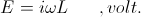
As an example is the condition where the E.M.F., E, is the cause, and the Current, i, is the effect,
The Proportionality, R, exists between Cause, E, and Effect, i, and here it is a Resistance. If the Cause, E, is given graphically as a vertical co-ordinate, the resulting Load Line is the graphical plot of the Proportionality between the Cause, E, and the Effect, i.
For the condition of a constant fixed resistance, R, in Ohm the Load Line is a straight line. The slope of this line is the instantaneous ratio of the E.M.F. to the Current, and it is constant anywhere along the line. No differential relation exists in that the ratio of any E.M.F. to its co-responding current is always the same value. It is a constant resistance, R.
This is known as a Linear relationship.
(2) Electrical devices such as Incandescent Lamps or Thyrites do not exhibit a direct relation between cause and effect. For example, the Lamp shows and Increasing Resistance for and Increasing Current, and a Thyrite shows a decreasing Resistance for an increasing applied E.M.F. Here the Load Line is no longer straight, but it is now curved in a parabolic form. The slope is no longer constant but varies with position along the curve. An E.M.F. and its co-responding Current have a different ratio than another E.M.F. and Current taken at another point on the curve. The variation of the slope represents the variation of Resistance,
Cause and Effect are now in Dis-Proportion to each other. Here Effect can become exaggerated by the cause and a sine wave of E.M.F. no longer gives rise to a sine wave of Current, distortion results. This is known as a Non-Linear relationship. Magnetic Saturation in Magnetic material is one such disproportional relationship, here between the M.M.F. and the Magnetic Induction, the Load Lines are known as the Saturation Curves of the Magnetic Material.
In both the Linear and the Non-Linear relation every E.M.F. has one and only one co-responding current. These exist at one unique point on the Proportionality Curve. The Relationship here is Uni-Valent, or single valued.
(3) Another more complex relation can exist between Cause, E, and Effect, i. In this relationship Cause and Effect become Dis-Joint. Here the curve for rising values is not the same curve as for falling values. In this situation the graphical expressions of the relation is no longer Linear, nor is it non-Linear, it is now an Elliptical relationship. In the Non-Linear relationship the limit in curvature is the straight line, here the curvature is Infinitesimal. Likewise for the Elliptical relationship, the limit in ellipticity is the full circle, a limiting case for Elliptical curvature. When the “Load Line” is a circle the Proportionality Factor of Resistance becomes the Dis-Proportionality Factor of Reactance.
Reactance is Resistance in constant variation at an angular rate of . Here the Resistance is the Reaction of the Inductance to the constantly variable current,

(4) For the condition of the Elliptical Load Line, the point by point relationship is no longer uni-valent, for each Cause, or E.M.F., E, there exist two co-responding Effects, or Currents, i. These two Effects exist displaced in Time. Likewise, for each Effect, Current, i, there exists two co-responding Causes, E.M.F.s. These two Causes exist displaced in Time. Where it is the Linear or Non-Linear relationship is a Uni-Valent function, it is for the Circular and Elliptical relationships a Quadra-Valent function.
For the condition of the Linear and the Non-Linear relationships, As the Cause, or E.M.F. becomes smaller and smaller, likewise the Effect or Current becomes smaller and smaller. For both Proportionate and Dis-Proportionate relationships a zero Cause has a co-responding zero Effect. Both become zero together, Uni-Valent.
For the condition of the Circular and Elliptical relationships, these Quadra-Valent functions arrive at zero points in four locations on the curve, two for the Cause, E.M.F. and two for the Effect, Current. The two zero points for E.M.F. are displaced in Time as are the two zero points for Current, and all four zeros are displaced in Time from each other. Moreover here exists a unique situation where a Cause, E.M.F. can have zero Effect, Current, or and Effect, Current, can have no Cause, E.M.F. Cause and Effect are here Dis-Joint from each other. This condition can be called the Hysteretic Cycle of Proportionality.
(5) In its most general form, ruling out Non-Linearity, the Load Line can be considered a Circle rotating on an axis, this axis in the plane of the Circle and normal to its curvature, bisecting it. As this circle is turned on its axis it begins to contract into an ellipse. Continuing the rotation further, upon reaching one quadrant, 90 degrees, of rotation, the circle has completely contracted into a line with a slope of one, a 45 degree line. This quadrantal rotation represents the transformation from Reactance to Resistance. The angle by which the circle is displaced towards the line is called the Angle of Hysteresis, .
In order to carry the angle, , beyond one quadrant one more transformation is required. Here the circle has a pair of rotational axes, these also in a quadrature relation, dividing the circle into four quadrants. As the angle, , passes beyond 90 degree the rotational axis is shifted to the quadrantal axis and it is inverted. As the line opens into an ellipse the position of this curve now travels in the opposite direction, the A.C. wave now rotates around the Load-Line in the opposite direction. Continuing to advance angle, , another 90 degrees, upon reaching two quadrants the line has opened up again into a full circle with a cyclic direction opposite to the circle at the start when the angle, , was zero. This now is a Negative Reactance. Where the first quadrant of rotation transformed Reactance into Resistance, the second of rotation transforms Resistance into Negative Reactance. Continuing to carry the rotational, or Hysteretic Angle, , beyond two quadrants, or 180° degrees, again contracts this counter-circle back into an ellipse. However the slope of this ellipse is now backwards, or negative, this as well as counter-cyclic. Upon reaching the next quadrant of rotation the ellipse has contracted into a line but now the line has a negative slope. Here is the unique situation where an increasing Cause, E.M.F. has a co-responding decreasing Effect, Current. Inversely, it is the greater the Effect, the less the Cause required to produce this Effect. This is a condition of Negative Resistance.
Upon passing thru this inverse Linear relationship the rotational axis of the Load Line Circle is shifted back to the original. As angle, , is carried past three quadrants, or 270 degrees, the Load Line again opens into a Ellipse of positive slope and normal rotation. Continued rotation returns the Load Line back to the original circle of Reactance at four quadrants or 360 degrees.
(6) In symbolic form, for the four quadrants thru which the Angle of Hysteresis is rotated it is


Here the Versor Operator,  , expressed the Angle of Hysteresis, , in quadrantal form.
In any intermediate angle between quadrantal angles of 0, 90, 180, 270, the values of Reactance and Resistance combine in a quadrantal vector relationship, this for intermediate angles in the first quadrant the relation is given as,

This is the Hysteretic Impedance for the first quadrant, and
Here,  , is a Positive Impedance but now the Resistance has become an imaginary quantity. Likewise for the opposing quadrant the relation is given as,

Or by resolving powers of , it is

Here it is a negative Hysteretic Impedance. Hence Reactance and Resistance can be synthesized in Positive or Negative forms by positioning the Angle of Hysteresis, .
BK DE N6KPH
(1) Magnetic materials such as Iron exhibit internal parameter variations during a Magnetic cycle of Induction. These can be divided into two distinct phenomena, Saturation and Hysteresis. It has become commonplace to consider the two as a single phenomena, but this leads to misleading concepts. Saturation and Hysteresis must be analyzed separately.

Parameter variation of Inductance by external means, thru rotation or controlled saturation, can be utilized to develop synthesized Saturation and Hysteresis curves unique from those of the Iron itself. The practical knowledge in this realm is very limited. Experimentation is required here.
The principle apparatus utilizing parameter variation are the developments of Ernst Alexanderson, the Variable Induction Alternator


(3) C.P. Steinmetz, in his editions of “Theory and Calculation of A.C. Phenomena”, does not development Saturation and Hysteresis as separate and distinct phenomena. Saturation and Hysteresis are combined in the Magnetic material giving rise to a Distortion Complex of phase shifted harmonics. This is a composite of the separate amplitude and phase distortions. Little is given in the A.C. book that relates to the utilization of parameter variation for the generation of Electro-Motive Force and the transfer of Electric Energy thereby. Steinmetz only considers situations where Saturation and Hysteresis are considered as parasitic phenomena, these to be minimized. In later chapters, “Reaction Machines” and “Distortion of Waveshape and Its Causes”, Steinmetz develops an analysis of parameter variation and the E.M.F.s developed thereby.
A considerable portion of the Steinmetz A.C. book is devoted to the Synchronous Machine,


If the Field Current (and excitation) is increased beyond the value required for a neutral condition, the rotor pushes ahead of the rotating A.C. wave to a position advancedin phase, but still rotating in synchronism with the wave. With increasing excitation the machine begins to draw a leading Current from the power line, the greater the excitation, the greater the current taken by the machine from the line. Since these Currents are reactive no Energy is expended in maintaining them. Here the Synchronous Machine is exhibiting the characteristics of and Electro-Static Condenser and in this manner of operation it is called a Synchronous Condenser.
Inversely, reducing the Field Current below that required to maintain a neutral condition, the rotor falls behind the A.C. wave of the stator, this to a position retarded in phase while rotating with the A.C. wave. The less the excitation, the more the rotor lags behind the stator. With decreasing excitation the Machine draws a lagging Current from the power line, the less the excitation, the more Current is drawn. Here the machine is exhibiting the characteristics of a Reactance Coil. This can be called a Synchronous Reactor.
In this manner the Synchronous Machine is operating as a two terminal Reactance Arm. There is no connection to the rotating shaft. The Machine can synthesize an actual Inductor or Condenser. Operating in this manner the machine can create a substantial reactive power flow, this flow controlled by the D.C. excitation of the machine. ThisControlled Reactance is used at the end of long distant power lines in order to regulate the voltage and phase at lines end.
As a reactance arm the two terminals (per phase) serve as input and serve as output. There is only one power line. The Energy flows into the machine during one part of the Cycle, and Energy flows out of the machine during another part of the Cycle. Here input and output are separated in Time rather than space. The Energy is caught in a Hysteresis Loop.
It is important to note here that this machine is operating as a Synthesizer. The power flow of Condensers and Reactors are developed by synthesis, without the intense Dielectric and Magnetic Fields that normally are required to create this flow, or surging, of Electric Energy. Here a “Synthetic Power” is derived from a dynamic of parameter variational form.
BK DE N6KPH
In the chapter “Reaction Machines” Steinmetz continues with a more in depth analysis of parametric E.M.F. production. Here Steinmetz presents a situation where a Synchronous Machine can synthesize its own D.C. excitation. This is with no outside source of current to develop the M.M.F., nor any remnant Magnetism.
(2) The chapter “Reaction Machines” gives a more theoretical analysis of Hysteresis. Here the Hysteresis is no longer connected with Saturation, it is independently synthesized by the machine. A pair of Hysteresis Cycles can be formed, one is a forward cycle representing Energy consumption, the other is a reverse cycle representing Energy production; see hysteresis motor.
It is assumed thru the Law of Energy Continuity that the rotating shaft transfers the Energy that is produced or consumed in an Electrical form. The E.M.F. developed in the parametric machine however is unlike that developed by the Motor-Generator. The Motor-Generator is a Constant Magnetism machine and the energy transferred is strictly a function of shaft rotation. The regulation here between mechanical and electrical forms is definitely established by the Law of Energy Continuity.
The parametric E.M.F. is developed by a variation of Magnetism, it is not constant, but pulsates with respect to time. In this situation the machine operates in the constant Current condition and the Energy transferred is a function of Inductance variation via shaft rotation, but not shaft rotation directly. This complicates the Law of Energy Continuity.
(3) In the Synchronous Machine irregularities in pole facings and winding distributions give rise to a pulsation upon the normally constant Magnetism. This constancy is a characteristic of operation as a Motor-Generator. The E.M.F. of rotation and the E.M.F. of variation combines with it to give an effective total E.M.F. at the machine terminals.
Steinmetz suggests no apparatus for developing an E.M.F. by parametric means in his A.C. books, however the Alexanderson Alternator was under development at the time of writing of the Fifth Edition, 1916. In general these parametric variations in rotating machinery are hereby considered parasitic phenomena, just as with Saturation and Hysteresis in magnetic material. These effects are to be minimized not optimized. It is however in this series of writings that the optimization of parametric E.M.F. generation is sought, and its application to the Law of Energy Continuity studied.
(4) In the next chapter, “Distortion of Waveshape and Its Causes”, Steinmetz further develops the analysis of Synchronous Parameter Variation. The material presented in this chapter is minimal. Dimensional in-congruities, irrational units, ambiguous equations, and typo errors render the understanding of this chapter difficult. Also, again Saturation and Hysteresis become merged into a common phenomena, this blurring the true relations between Amplitude and Phase distortions.
In “Distortion of Waveshape and Its Causes” Steinmetz also gives an analysis of the synchronous parameter variation of Resistance, such as in Arc Lighting Systems. Here the remarkable condition exists that a form of reactive power is produced, however with no phase displacement. It is noted by Steinmetz that, where it is Inductance variation gives rise to an effective Resistance of Energy transfer, here the Resistance variation gives rise to an effective Reactance of Energy storage. This reactance is synthetic, no Field of Induction, nor relative mechanical activity, is present to facilitate any reactive power. This synthetic reactance is a result of the particular cause and effect relations in the variant resistance. Again the Law of Energy Continuity is in question. Here the Law of Energy Perpetuity may even be invalidated. This is an important study.
(5) The chapter 25 from “Theory and Calculation of Alternating Current Phenomena” Fifth Edition, 1916, is here re-developed in the following, concentrating of a general equation for the synchronous parameter variation of Inductance and the E.M.F. developed thereby. Symbol standardization, and rationalizing by removal of pi and root two, will be applied to the expressions of Steinmetz.
The parameter variation in this chapter is of the synchronous type. Here the Inductance of a reactance coil with an applied A.C. current is brought into synchronous variation at a harmonic rate in proportion to that of the applied A.C. current. Two E.M.F.’s are developed, that of the reactance opposing the variation of Current, and that of Inductance variation. The E.M.F. of constant Inductance and Current variation is compounded with the E.M.F. of constant Current and Inductance variation. Steinmetz fails to separated these two E.M.F’s. Here exists a modulation process, the Inductance variation modulating the reactance current variation. Complex E.M.F.’s result consisting of multiple frequencies and with distorted waveforms.
In chapter 25, expressions are given for the E.M.F. of rotating parameter variation, as in the Synchronous Machine, and the E.M.F. of stationary parameter variation, as in the magnetic material of the static reactance coil. The two are of basically the same mathematical form thus distinction is not a necessity in the development of a General Equation of synchronous parameter variation.
Chapter 25, article 234 begins the analysis, “Lack of Uniformity and Pulsations of the Magnetic Field.” This serves as the basis for the derived General Equation. The sine wave of Magnetism is given by,
Where,

And

Here the Time Angle is the independent variable, this is defined by,
And

Where,
F, frequency in cycles/sec,
and
t, Time variable, seconds.
This time angle is a dimensionless position variable on the A.C. cycle of revolution. Substituting the cyclic period,
Gives the Time Angle as the ratio of the time along the cycle to the time of a complete cycle, that is,
Or in rational form, in radian,
Where,

Where,


Substituting the following relation for Magnetic Induction,

Into the general expression segregates the two subjects of parameter variation, that of the Current, i, and that of the Inductance, L. The sine wave of current is given by,
And the pulsating wave of Inductance is given by,

Here in the Inductance the sine wave of variation is offset, and for a modulation depth of one (100%) the sine wave is a pulsating wave in variation with peaks at zero and twice the value of static Inductance. This is expressed as

Where

Is the sine wave of Inductance variation. For a modulation depth of zero the cosine term vanishes and the constant term of static Inductance, L, remains,
Segregating variations the General Equations for Magnetic synchronous parameter variation becomes,

(7) For the condition of Saturation and Hysteresis as exists in magnetic materials the process of saturation is the same for positive and negative half cycles, it is symmetrical. The reduction of Inductance due to saturation in the positive half is the same reduction of Inductance due to the saturation in the negative half. Hence the reduction, or modulation, of Inductance is at Twice the frequency of the A.C. cycle of Magnetism, that is, the Inductance pulsates at Double Frequency. In this situation it is,
n = 2 , numeric,
Where, n, is the harmonic number.
, the angle of hysteresis, and Saturation gives rise to a modulation factor,  , the depth of modulation. Hence the sine wave of Inductance variation is expressed by the term,

This for Magnetic material.
(8) The E.M.F. developed by the instantaneous Magnetic Induction,  , is the time rate of its variation,
The time rate of variation is expressed as,
Steinmetz substitutes the expression for angular rate of variation,
Where,
And
This angular differential is here given symbolically,
And it is dimensionless. Here gamma represents an infinitesimal Versor Operator, this of an infinite number of divisions, symbolically,
Here the angular frequency, , has become a tensor magnitude, or a Tensor Frequency. The angular rate of variation is thus symbolically expressed by,
Substituting into the relation for E.M.F. gives,

And differentiating, gives the developed E.M.F. of synchronous parameter variation of Inductance as,

A1 being the Lower Sideband Amplitude, and
A2 being the Upper Sideband Amplitude. Also,

The Lower Sideband Time Angle,

The Upper Sideband Time Angle.
Note here that

Dimensionally establishes the volt.
Hence a pair of new Frequencies are generated by the synchronous parameter variation of Inductance, these given by the relations,
Lower Sideband Frequency,

Upper Sideband Frequency,

Where, , is the “Carrier Frequency”, of current variation via the A.C. cycle of the external current source.
Hence three alternating electric waves exist in the process of synchronous parameter variation, the values are given in Table 1,

(9) Steinmetz does not develop this subject much further. The equations for parameter variation in stationary reactance coils, article 236, are dimensionally invalid,
A weber is not an ohm-second per radian, it is rightly given as
The equations for harmonic summation are not clear and something seems not right. No in depth analysis exists of Resistance parameter variation on a theoretical level, everything is reduced to effective values. E.M.F. is not equated to a co-responding current in many cases making the study of Power Flow difficult in the case of Inductance parameter variation. It is noteworthy in this chapter that Steinmetz gives experimental verification of his parameter variation expressions. It is this feature of Steinmetz’s work that makes it of value.
(10) Herewith closes this series of writings, “The Law of Electro-Magnetic Induction”. Three principle conditions for the development of electro-motive force have been presented,
Constant Magnetism,
Constant Current,
Constant Inductance.
While the condition of Constant Magnetism, the Motor-Generator, and the condition of Constant Inductance, the Reactance Coil, are well known engineering realities, it is the special condition of Constant Current that awaits further analysis and experimentation. In this particular condition of E.M.F. development the Law of Energy Continuity may be in need of re-definition. Here the Law of Energy Perpetuity, the holy dictum of modernistic physics, may possibly be invalidated.
73 DE N6KPH SK…..